All documentation links
ProActive Workflows & Scheduling (PWS)
-
PWS User Guide
(Workflows, Workload automation, Jobs, Tasks, Catalog, Resource Management, Big Data/ETL, …) PWS Modules
Job Planner
(Time-based Scheduling)Event Orchestration
(Event-based Scheduling)Service Automation
(PaaS On-Demand, Service deployment and management)
PWS Admin Guide
(Installation, Infrastructure & Nodes setup, Agents,…)
ProActive AI Orchestration (PAIO)
PAIO User Guide
(a complete Data Science and Machine Learning platform, with Studio & MLOps)
1. Overview
1.1. What is ProActive AI Orchestration (PAIO)?
ProActive AI Orchestration (PAIO) is a complete DSML platform (Data Science and Machine Learning) including a ML Studio, AutoML, Data Science Orchestration and MLOps for the deployment, training, execution and scalability of artificial intelligence and machine learning models on any type of infrastructure. Created for data scientists and ML engineers, the solution is simple to use and accelerate the development and deployment of machine learning models.
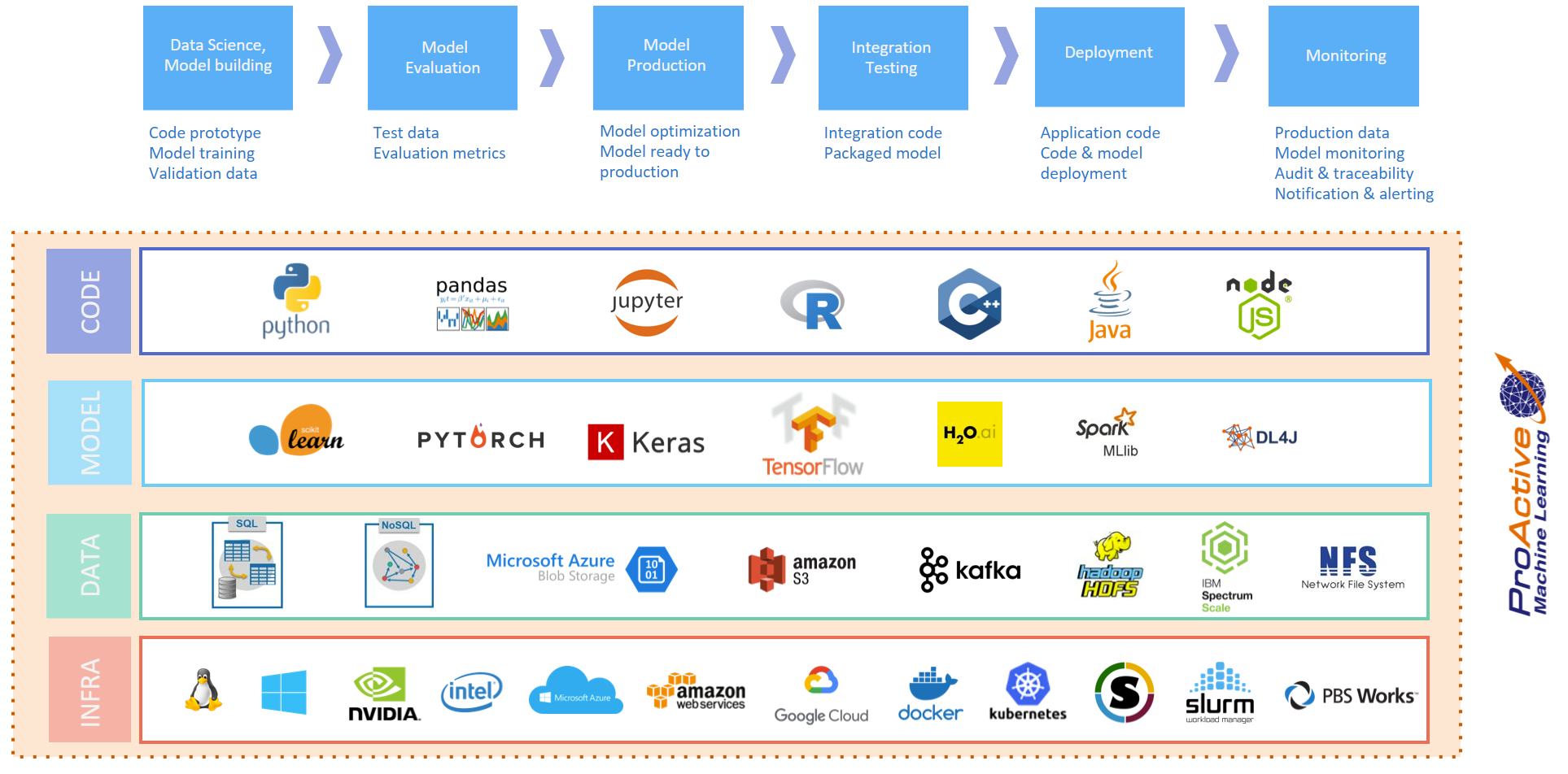
ProActive AI Orchestration platform provides a rich catalog of generic machine learning tasks that can be connected together to build either basic or advanced machine learning workflows for various use cases such as: fraud detection, text analysis, online offer recommendations, prediction of equipment failures, facial expression analysis, etc. PAIO workflows enable users to manage machine learning pipelines through the different phases of the development lifecycle and allow them to better control tasks parallelization, by running the tasks on resources matching constraints (Multi-CPU, GPU, FPGA, data locality, libraries, etc).
The ProActive AI Orchestration platform is an open source solution, and it can be tested online without installation on our try platforms here.
The MLOps Dashboard is a centralized platform that streamlines the management and monitoring of AI model deployments. It offers a detailed overview of deployment pipelines, real-time performance metrics allowing for efficient oversight of models and servers in production. The dashboard also tracks CPU and GPU resource usage for both individual models and the entire platform, ensuring optimal performance. Additionally, it includes robust functionalities for detecting and managing data drift, helping users maintain the accuracy and reliability of deployed models over time.
Refer to MLOps Dashboard section for more information.
1.2. Glossary
The following terms are used throughout the documentation:
- ProActive Workflows & Scheduling
-
The full distribution of ProActive for Workflows & Scheduling, it contains the ProActive Scheduler server, the REST & Web interfaces, the command line tools. It is the commercial product name.
- ProActive Scheduler
-
Can refer to any of the following:
-
A complete set of ProActive components.
-
An archive that contains a released version of ProActive components, for example
activeeon_enterprise-pca_server-OS-ARCH-VERSION.zip. -
A set of server-side ProActive components installed and running on a Server Host.
-
- Resource Manager
-
ProActive component that manages ProActive Nodes running on Compute Hosts.
- Scheduler
-
ProActive component that accepts Jobs from users, orders the constituent Tasks according to priority and resource availability, and eventually executes them on the resources (ProActive Nodes) provided by the Resource Manager.
| Please note the difference between Scheduler and ProActive Scheduler. |
- REST API
-
ProActive component that provides RESTful API for the Resource Manager, the Scheduler and the Catalog.
- Resource Manager Web Interface
-
ProActive component that provides a web interface to the Resource Manager.
- Scheduler Web Interface
-
ProActive component that provides a web interface to the Scheduler.
- Workflow Studio
-
ProActive component that provides a web interface for designing Workflows.
- ProActive AI Orchestration
-
PAIO component that provides a web interface for designing and composing ML Workflows with drag and drop.
- Job Planner Portal
-
ProActive component that provides a web interface for planning Workflows, and creating Calendar Definitions
- Job Planner
-
A ProActive component providing advanced scheduling options for Workflows.
- Bucket
-
ProActive notion used with the Catalog to refer to a specific collection of ProActive Objects and in particular ProActive Workflows.
- Server Host
-
The machine on which ProActive Scheduler is installed.
SCHEDULER_ADDRESS-
The IP address of the Server Host.
- ProActive Node
-
One ProActive Node can execute one Task at a time. This concept is often tied to the number of cores available on a Compute Host. We assume a task consumes one core (more is possible, so on a 4 cores machines you might want to run 4 ProActive Nodes. One (by default) or more ProActive Nodes can be executed in a Java process on the Compute Hosts and will communicate with the ProActive Scheduler to execute tasks. We distinguish two types of ProActive Nodes:
-
Server ProActive Nodes: Nodes that are running in the same host as ProActive server;
-
Remote ProActive Nodes: Nodes that are running on machines other than ProActive Server.
-
- Compute Host
-
Any machine which is meant to provide computational resources to be managed by the ProActive Scheduler. One or more ProActive Nodes need to be running on the machine for it to be managed by the ProActive Scheduler.
|
Examples of Compute Hosts:
|
PROACTIVE_HOME-
The path to the extracted archive of ProActive Scheduler release, either on the Server Host or on a Compute Host.
- Workflow
-
User-defined representation of a distributed computation. Consists of the definitions of one or more Tasks and their dependencies.
- Generic Information
-
Are additional information which are attached to Workflows.
- Job
-
An instance of a Workflow submitted to the ProActive Scheduler. Sometimes also used as a synonym for Workflow.
- Job Icon
-
An icon representing the Job and displayed in portals. The Job Icon is defined by the Generic Information workflow.icon.
- Task
-
A unit of computation handled by ProActive Scheduler. Both Workflows and Jobs are made of Tasks.
- Task Icon
-
An icon representing the Task and displayed in the Studio portal. The Task Icon is defined by the Task Generic Information task.icon.
- ProActive Agent
-
A daemon installed on a Compute Host that starts and stops ProActive Nodes according to a schedule, restarts ProActive Nodes in case of failure and enforces resource limits for the Tasks.
2. Get Started
To submit your first Machine Learning (ML) workflow to ProActive Scheduler, install it in your environment (default credentials: admin/admin) or just use our demo platform try.activeeon.com.
ProActive Scheduler provides comprehensive interfaces that allow to:
-
Create workflows using ProActive Workflow Studio
-
Submit workflows, monitor their execution and retrieve the tasks results using ProActive Scheduler Portal
-
Add resources and monitor them using ProActive Resource Manager Portal
-
Version and share various objects using ProActive Catalog Portal
-
Provide an end-user workflow submission interface using Workflow Execution Portal
-
Generate metrics of multiple job executions using Job Analytics Portal
-
Plan workflow executions over time using Job Planner Portal
-
Add services using Service Automation Portal
-
Perform event based scheduling using Event Orchestration Portal
-
Control manual workflows validation steps using Notification Portal
We also provide a REST API and command line interfaces for advanced users.
3. Create a First Predictive Solution
Suppose you need to predict houses prices based on this information (features) provided by the estate agency:
-
CRIM per capita crime rate by town
-
ZN proportion of residential lawd zoned for lots over 25000
-
INDUS proportion of non-retail business acres per town
-
CHAS Charles River dummy variable
-
NOX nitric oxides concentration
-
RM average number of rooms per dwelling
-
AGE proportion of owner-occupied units built prior to 1940
-
DIS weighted distances to five Boston Employment centres
-
RAD index of accessibility to radial highways
-
TAX full-value property-tax rate per $10 000
-
PTRATIO pupil-teacher ratio by town
-
B 1000(Bk - 0.63)^2 where Bk is the proportion of blacks by town
-
LSTAT % lower status of the population
-
MDEV Median value of owner-occupied homes in $1000' s
Predicting houses prices is a complex problem, but we can simplify it a bit for this step-by-step example. We’ll show you how you can easily create a predictive analytics solution using PAIO.
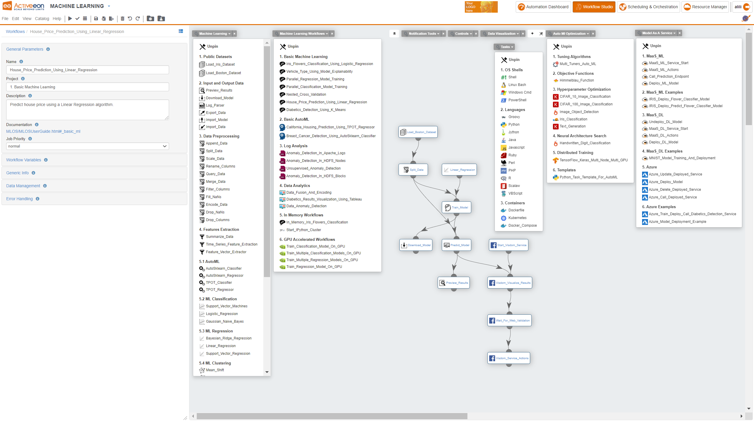
3.1. Manage the Canvas
To use PAIO, you need to select the Machine Learning preset as main catalog in the ProActive Studio. This preset contains a set of buckets containing machine learning tasks and workflows that enables you to upload and prepare data, train a model and test it.
-
Open ProActive Workflow Studio home page.
-
Create a new workflow.
-
Change palette preset to
Machine Learning. -
Click on
ai-machine-learningcatalog and pin it open, and same for theai-data-visualizationcatalog. -
Organize your canvas.
| Change palette preset allows the user to visualise different set of catalogs in the studio. |
3.2. Upload Data
To upload data into the Workflow, you need to use a dataset stored in a CSV file.
-
Once dataset has been converted to CSV format, upload it into a cloud storage service for example Amazon S3. For this tutorial, we will use Boston house prices dataset available on this link: https://s3.eu-west-2.amazonaws.com/activeeon-public/datasets/boston-houses-prices.csv
-
Drag and drop the Import_Data task from the
ai-machine-learningbucket in the ProActive AI Orchestration. -
Click on the task and click
General Parametersin the left to change the default parameters of this task. -
Put in FILE_URL variable the S3 link to upload your dataset.
-
Set the other parameters according to your dataset format.
This task uploads the data into the workflow that we can for model training and testing.
If you want to skip these steps, you can directly use the Load_Boston_Dataset Task by a simple drag and drop.
3.3. Prepare Data
This step consists of preparing the data for the training and testing of the predictive model. So in this example, we will simply split our datset into two separate datasets: one for training and one for testing.
To do this, we use the Split_Data Task in the machine_learning bucket.
-
Drag and drop the Split_Data Task into the canvas, and connect it to the Import_Data or Load_Boston_Dataset Task.
-
By default, the ratio is 0.7 this means that 70% of the dataset will be used for training the model and 0.3 for testing it.
-
Click the Split_Data Task and set the TRAIN_SIZE variable to 0.6.
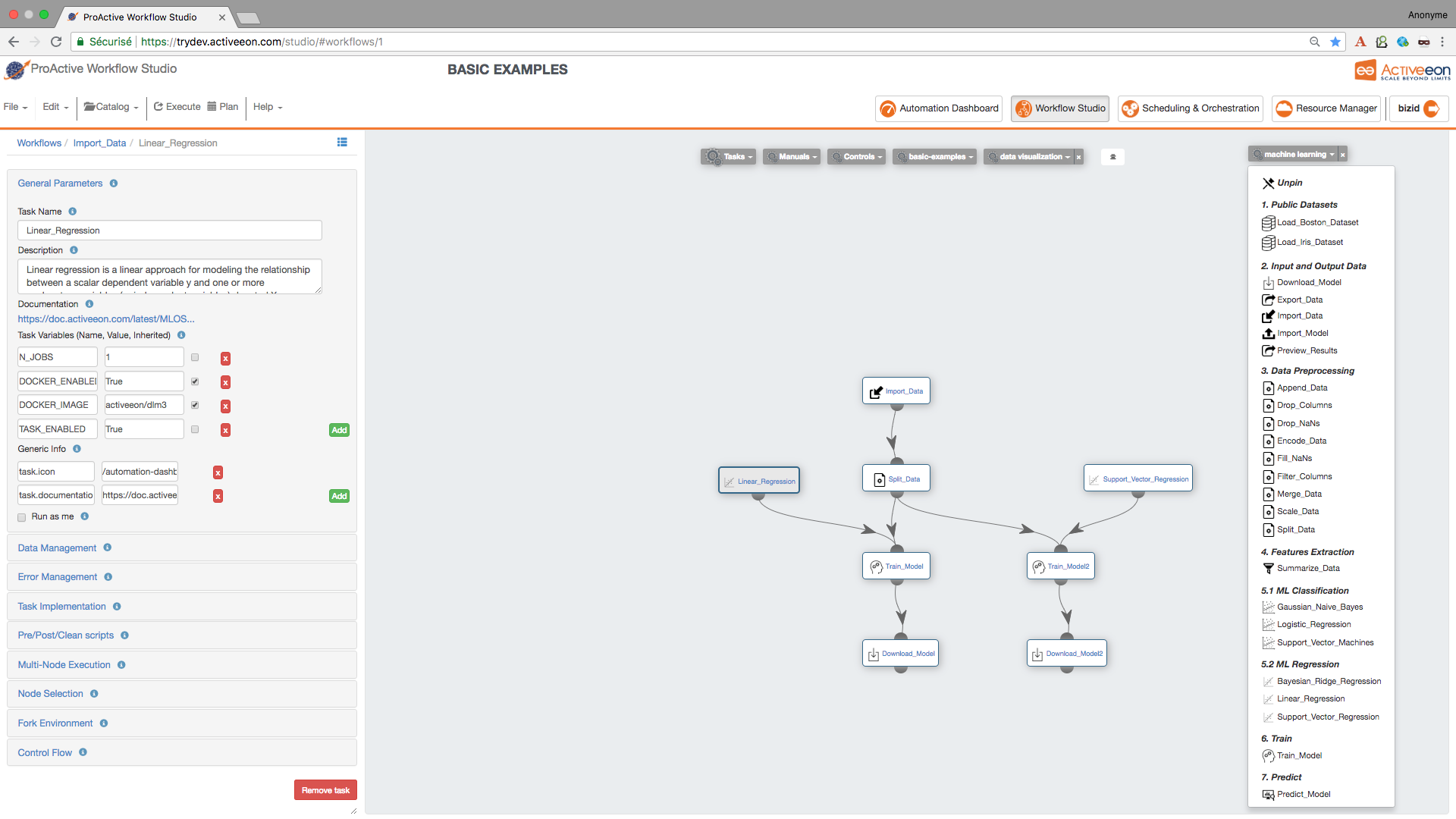
3.4. Train a Predictive Model
Using PAIO, you can easily create different ML models in a single experiment and compare their results. This type of experimentation helps you find the best solution for your problem.
You can also enrich the ai-machine-learning bucket by adding new ML algorithms and publish or customize an existing task according to your requirements as the tasks are open source.
To change the code of a task click on it and click the Task Implementation. You can also add new variables to a specific task.
|
In this step, we will create two different types of models and then compare their scores to decide which algorithm is most suitable to our problem. As the Boston dataset used for this example consists of predicting price of houses (continuous label). As such, we need to deal with a regression predictive problem.
To solve this problem, we have to choose a regression algorithm to train the predictive model. To see the available regression algorithms available on the PAIO, see ML Regression Section in the ai-machine-learning bucket.
For this example, we will use Linear_Regression Task and Support_Vector_Regression Task.
-
Find the Linear_Regression Task and Support_Vector_Regression Task and drag them into the canvas.
-
Find the Train_Model Task and drag it twice into the canvas and set its LABEL_COLUMN variable to LABEL.
-
Connect the Split_Data Task to the two Train_Model Tasks in order to give it access to the training data. Connect then the Linear_Regression Task to the first Train_Model Task and Support_Vector_Regression to the second Train_Model Task.
-
To be able to download the model learned by each algorithm, drag two Download_Model Tasks and connect them to each Train_Model Task.
3.5. Test the Predictive Model
To evaluate the two learned predictive models, we will use the testing data that was separated out by the Split_Data Task to score our trained models. We can then compare the results of the two models to see which generated better results.
-
Find the Predict_Model Task and drag and drop it twice into the canvas and set its LABEL_COLUMN variable to LABEL.
-
Connect the first Predict_Model Task to the Train_Model Task that is connected to Support_Vector_Regression Task.
-
Connect the second Predict_Model Task to the Train_Model Task that is connected to Linear_Regression Task.
-
Connect both Predict_Model Tasks to the Split_Data Task.
-
Find the Preview_Results Task in the ML bucket and drag and drop it twice into the canvas.
-
Connect each Preview_Results Task with Predict_Model.
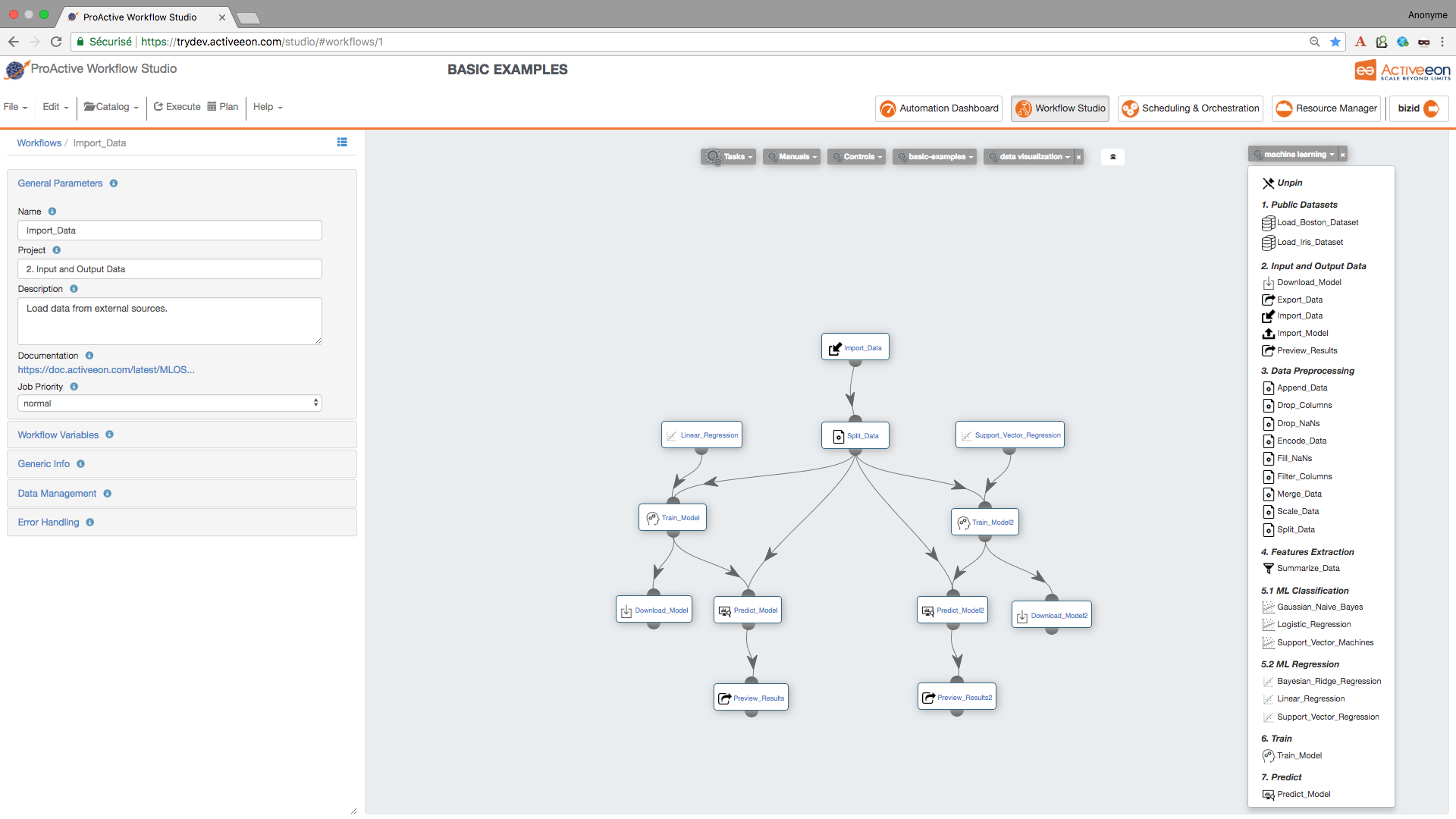
| if you have a pickled file (.pkl) containing a predictive model that you have learned using another platform, and you need to test it in the PAIO, you can load it using Import_Model Task. |
3.6. Run the Experiment and Preview the Results
Now the workflow is completed, let’s execute it by:
-
Click the Execute button on the menu to run the workflow.
-
Click the Scheduling & Orchestration button to track the workflow execution progress.
-
Click the Visualization tab and track the progress of your workflow execution (a green check mark appears on each Task when its execution is finished).
-
Visualize the output logs by clicking on the output tab and check the streaming check box.
-
Click the Tasks tab, select a Preview_Results task and click on the Preview tab, then click either on Open in browser to preview the results on your browser or on Save as file to download the results locally.
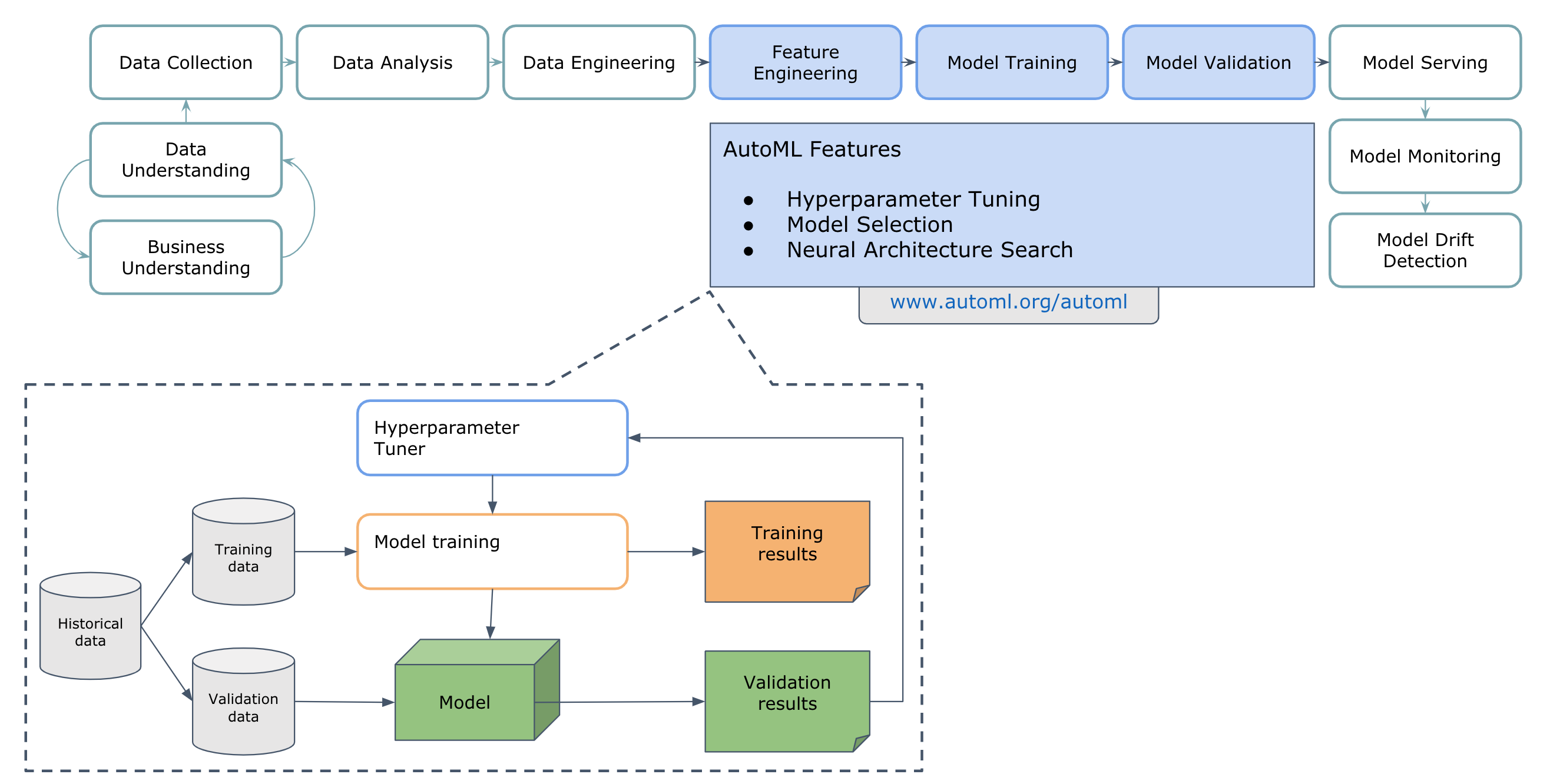
4. Automated Machine Learning (AutoML)
The ai-auto-ml-optimization bucket contains the Distributed_Auto_ML workflow that can be easily used to find the operating parameters for any system whose performance can be measured as a function of adjustable parameters.
It is an estimator that minimizes the posterior expected value of a loss function.
This bucket also comes with a set of workflows' examples that demonstrates how we can optimize mathematical functions, PAIO workflows and machine/deep learning algorithms from scripts using AutoML tuners.
In the following subsections, several tables represent the main variables that characterize the AutoML workflows.
In addition to the variables mentioned below, there is a set of generic variables that are common between all workflows
which can be found in the subsection AI Workflows Common Variables.
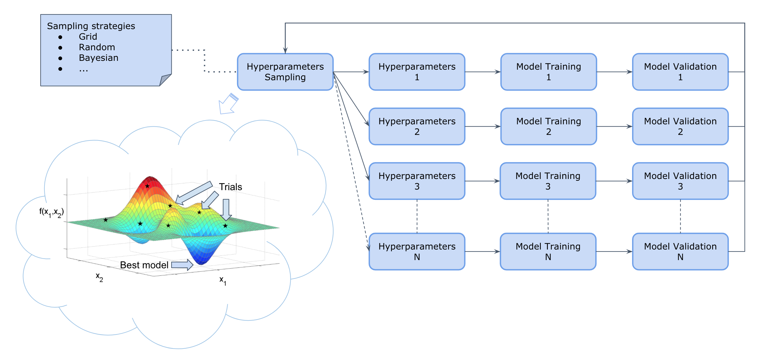
4.1. Distributed AutoML
The Distributed_Auto_ML workflow proposes six algorithms for distributed hyperparameters' optimization. The choice of the
sampling/search strategy depends strongly on the tackled problem.
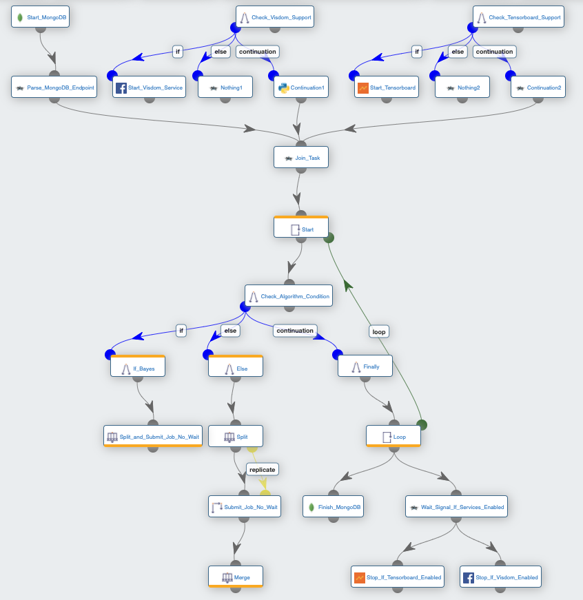
Distributed_Auto_ML workflow comes with specific pipelines (parallel or sequential) and visualization tools
(Visdom or TensorBoard) as described in the subsections below.
Variables:
Variable name |
Description |
Type |
|
Specifies the tuner algorithm that will be used for hyperparameter optimization. |
List [Bayes, Grid, Random, QuasiRandom, CMAES, MOCMAES] (default=Random) |
|
Specifies the number of maximum iterations. It should be an integer number higher than zero. Set |
Int (default=2) |
|
Specifies the number of parallel executions per iteration. It should be an integer number higher than zero. |
Int (default=2) |
|
Specifies the number of hyperparameter sampling repetitions. Ensures every experiment is repeated a given number of times. It should be an integer number higher than one. Set |
Int (default=-1) |
|
If higher than zero, pause the workflow after every specified number of iterations. Set |
Int (default=-1) |
|
If higher than zero, stop the workflow execution if loss is lower than the specified value. Set |
Int (default=-1) |
|
Specifies the workflow path from the catalog that should be optimized. |
String (default=ai-auto-ml-optimization/Himmelblau_Function) |
|
Name of the native scheduler node source to use on the target workflow tasks when deployed inside a cluster such as SLURM, LSF, etc. |
String (default=empty) |
|
Parameters given to the native scheduler (SLURM, LSF, etc) while requesting a ProActive node used to deploy the target workflow tasks. |
String (default=empty) |
|
If not empty, the target workflow tasks will be run only on nodes that contains the specified token. |
String (default=empty) |
|
If not empty, the target workflow tasks will be run only on nodes belonging to the specified node source. |
String (default=empty) |
|
Specifies the container platform to be used for executing the target workflow tasks. |
List [no-container, docker, podman, singularity] (default=empty) |
|
Specifies the name of the container image that will be used to run the target workflow tasks. |
List [docker://activeeon/dlm3, docker://activeeon/cuda, docker://activeeon/cuda2, docker://activeeon/rapidsai, docker://activeeon/nvidia:rapidsai, docker://activeeon/nvidia:pytorch, docker://activeeon/nvidia:tensorflow, docker://activeeon/tensorflow:latest, docker://activeeon/tensorflow:latest-gpu] (default=empty) |
|
If True, it will activate the use of GPU for the target workflow tasks on the selected container platform. |
Boolean (default=empty) |
|
If True, it will activate the use of NVIDIA RAPIDS for the target workflow tasks on the selected container platform. |
Boolean (default=empty) |
|
If True, the Visdom service is started allowing the user to visualize the hyperparameter optimization using the Visdom web interface. |
Boolean (default=False) |
|
If True, requests to Visdom are sent via a proxy server. |
Boolean (default=False) |
|
If True, the TensorBoard service is started allowing the user to visualize the hyperparameter optimization using the TensorBoard web interface. |
Boolean (default=False) |
|
If True, requests to TensorBoard are sent via a proxy server. |
Boolean (default=False) |
How to define the search space:
This subsection describes common building blocks to define a search space:
-
uniform: Uniform continuous distribution.
-
quantized_uniform: Uniform discrete distribution.
-
log: Logarithmic uniform continuous distribution.
-
quantized_log: Logarithmic uniform discrete distribution.
-
choice: Uniform choice distribution between non-numeric samples.
Which tuner algorithm to choose?
The choice of the tuner depends on the following aspects:
-
Time required to evaluate the model.
-
Number of hyperparameters to optimize.
-
Type of variable.
-
The size of the search space.
In the following, we briefly describe the different tuners proposed by the Distributed_Auto_ML workflow:
-
Grid sampling applies when all variables are discrete, and the number of possibilities is low. A grid search is a naive approach that will simply try all possibilities making the search extremely long even for medium-sized problems.
-
Random sampling is an alternative to grid search when the number of discrete parameters to optimize, and the time required for each evaluation is high. Random search picks the point randomly from the configuration space.
-
QuasiRandom sampling ensures a much more uniform exploration of the search space than traditional pseudo random. Thus, quasi random sampling is preferable when not all variables are discrete, the number of dimensions is high, and the time required to evaluate a solution is high.
-
Bayes search models the search space using gaussian process regression, which allows an estimation of the loss function, and the uncertainty on that estimate at every point of the search space. Modeling the search space suffers from the curse of dimensionality, which makes this method more suitable when the number of dimensions is low.
-
CMAES search (Covariance Matrix Adaptation Evolution Strategy) is one of the most powerful black-box optimization algorithm. However, it requires a significant number of model evaluation (in the order of 10 to 50 times the number of dimensions) to converge to an optimal solution. This search method is more suitable when the time required for a model evaluation is relatively low.
-
MOCMAES search (Multi-Objective Covariance Matrix Adaptation Evolution Strategy) is a multi-objective algorithm optimizing multiple tradeoffs simultaneously. To do that, MOCMAES employs a number of CMAES algorithms.
Here is a table that summarizes when to use each algorithm.
Algorithm |
Time |
Dimensions |
Continuity |
Conditions |
Multi-objective |
|
|
|
|
|
|
|
|
|
|
|
|
|
|
|
|
|
|
|
|
|
|
|
|
|
|
|
|
|
|
|
|
|
|
|
|
4.2. Objective Functions
The following workflows represent some mathematical functions that can be optimized by the Distributed_Auto_ML tuners.
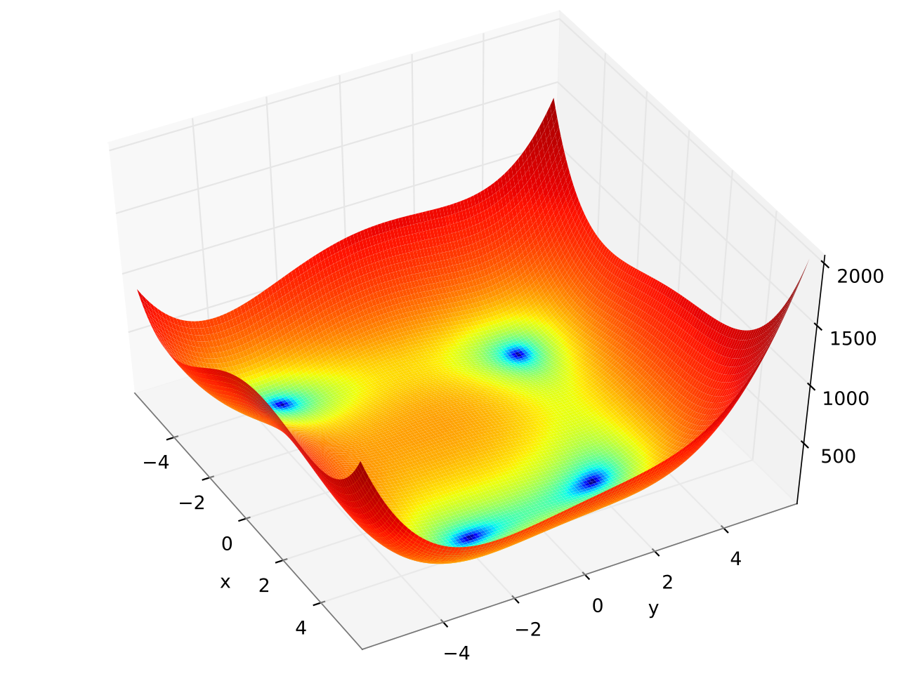
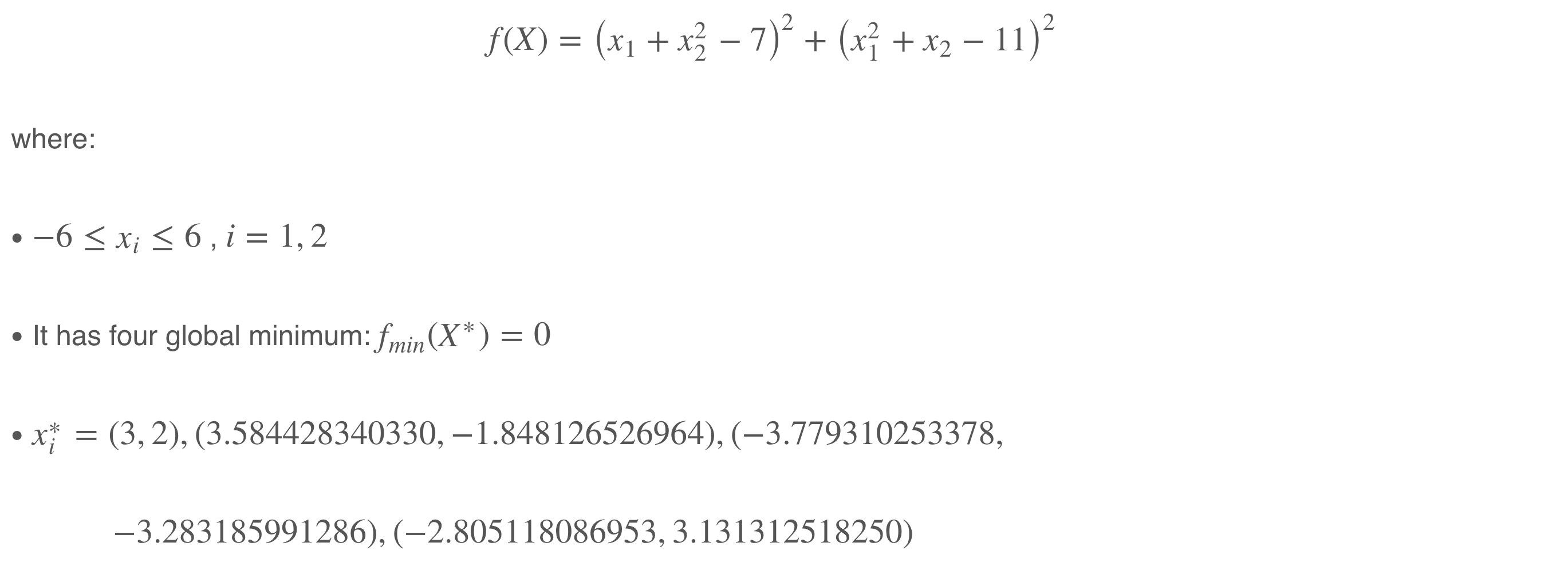
Himmelblau_Function: is a multi-modal function containing four identical local minima. It’s used to test the performance of optimization algorithms. For more info, please click here.
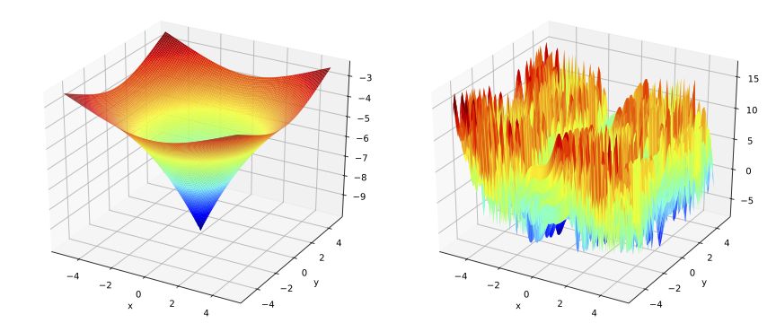
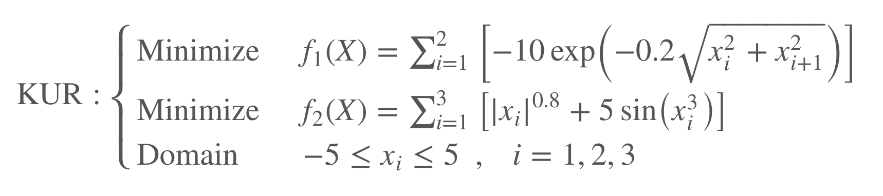
Kursawe_Multiobjective_Function: is a multiobjective function proposed by Frank Kursawe. It has two objectives (f1, f2) to minimize. For more info, please click here.
4.3. Hyperparameter Optimization
The following workflows represent some machine learning and deep learning algorithms that can be optimized.
These workflows have several common variables as in Distributed_Auto_ML. Some workflows are characterized
by few additional variables.
CIFAR_10_Image_Classification: trains a simple deep CNN on the CIFAR10 images dataset using the Keras library.
Variable name |
Description |
Type |
|
The number of times data is passed forward and backward through the training algorithm. |
Integer (default=3) |
|
A set of specific variables (usecase-related) that are used in the model training process. |
JSON format |
|
Specifies the representation of the search space which has to be defined using dictionaries or by entering the path of a json file stored in the catalog. |
JSON format |
|
Specifies the name to be provided for the instance. |
String (default=tensorboard-server) |
|
Specifies the path where the docker logs are created and stored on the docker container. |
String (default=/graphs/$INSTANCE_NAME) |
|
If True, the user will be able to run the workflow in a rootless mode. |
(default=True) |
The following workflows have common variables with the above illustrated workflows.
CIFAR_10_Image_Classification: trains a simple deep CNN on the CIFAR10 images dataset using the Keras library.
CIFAR_100_Image_Classification: trains a simple deep CNN on the CIFAR100 images dataset using the Keras library.
Image_Object_Detection: trains a YOLO model on the coco dataset using PAIO deep learning generic tasks.
Digits_Classification: python script illustrating an example of multiple machine learning models optimization.
Text_Generation: trains a simple Long Short-Term Memory (LSTM) to learn sequences of characters from 'The Alchemist' book. It’s a novel by Brazilian author Paulo Coelho that was first published in 1988.
4.4. Neural Architecture Search
The following workflows contain a search space containing a set of possible neural networks architectures that can be used by Distributed_Auto_ML to automatically find the best combinations of neural architectures within the search space.
Single_Handwritten_Digit_Classification: trains a simple deep CNN on the MNIST dataset using the PyTorch library. This example allows to search for two types of neural architectures defined in the Handwritten_Digit_Classification_Search_Space.json file.
Multiple_Objective_Handwritten_Digit_Classification: trains a simple deep CNN on the MNIST dataset using the PyTorch library. This example allows optimizing multiple losses, such as accuracy, number of parameters, and memory access cost (MAC) measure.
4.5. Distributed Training
The following workflows illustrate some examples of multi-node and multi-gpu distributed learning.
TensorFlow_Keras_Multi_Node_Multi_GPU: is a TensorFlow + Keras workflow template for distributed training (multi-node multi-gpu) with AutoML support.
TensorFlow_Keras_Multi_GPU_Horovod: is a Horovod workflow template that support multi-gpu and AutoML.
4.6. Templates
The following workflows represent python templates that can be used to implement a generic machine learning task.
Python_Task: is a simple Python task template pre-configured to run with Distributed_Auto_ML.
R_Task: is a simple R task template pre-configured to run with Distributed_Auto_ML.
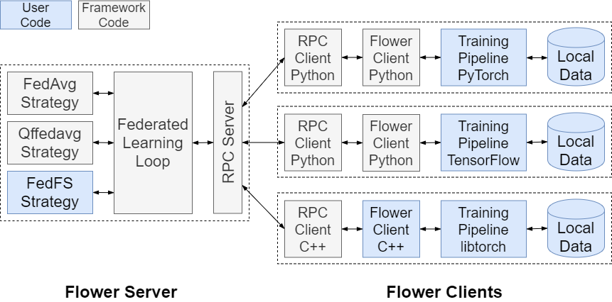
5. Federated Learning (FL)
Federated Learning (FL) enables to train an algorithm across multiple decentralized devices (or servers) holding local data samples, without exchanging them.
The ai-federated-learning bucket contains a few examples of Federated Learning workflows that can be easily used to build a common and robust machine learning model without sharing data, thus allowing to address critical issues such as data privacy, data security, data access rights and access to heterogeneous data.
This bucket uses the Flower library to implement federated learning workflows.
The Flower library is a friendly federated learning framework that presents a unified approach for federated learning.
It help federating any workload using any ML framework, and any programming language.
5.1. PyTorch Federated Learning Tasks
The following workflows represent a client/server templates that can be used to implement a Federated Learning workflow using PyTorch.
PyTorch_FL_Client_Task: is a Federated Learning Client task template using PyTorch.
PyTorch_FL_Server_Task: is a Federated Learning Server task template using PyTorch.
5.2. TensorFlow Federated Learning Tasks
The following workflows represent a client/server templates that can be used to implement a Federated Learning workflow using TensorFlow/Keras.
TensorFlow_FL_Client_Task: is a Federated Learning Client task template using TensorFlow/Keras.
TensorFlow_FL_Server_Task: is a Federated Learning Server task template using TensorFlow/Keras.
5.3. Federated Learning Workflows
The following workflows uses the federated learning to train a deep Convolutional Neural Network (ConvNet/CNN) on the CIFAR10 images dataset using the Flower library.
PyTorch_Federated_Learning_Example: shows an example of Federated Learning workflow using PyTorch.
TensorFlow_Federated_Learning_Example: shows an example of Federated Learning workflow using TensorFlow/Keras.
References:
6. MLOps Dashboard
In the domain of machine learning operations (MLOps), the successful deployment and continuous monitoring of machine learning models are crucial for ensuring their reliability and performance. However, in addition to managing models, it is equally important to handle the infrastructure where the models are deployed. This is where an MLOps dashboard, designed specifically for model serving and monitoring becomes a powerful asset.
An MLOps dashboard serves as a centralized hub for data scientists, engineers, and stakeholders involved in deploying and monitoring machine learning models. It provides a comprehensive view of the deployment pipelines and real-time performance metrics. Furthermore, it includes features specifically designed to manage and monitor the underlying model servers.
Model servers are responsible for hosting the deployed machine learning models and providing predictions or inferences to applications or users. An MLOps dashboard equipped with model server management capabilities allows users to seamlessly handle the infrastructure aspect of model deployment.
The MLOps dashboard extends its monitoring capabilities by incorporating the monitoring of the underlying infrastructure’s health and performance. It provides real-time insights into server metrics, resource utilization, and availability, allowing teams to promptly identify and address any infrastructure-related issues. This comprehensive monitoring capability ensures that the model servers are performing optimally and can handle the predicted workloads efficiently.
Collaboration is also a key aspect of an MLOps dashboard. It enables seamless communication and collaboration among data scientists, engineers, and other stakeholders involved in both model deployment and server management. The dashboard allows users to share insights, discuss server performance trends, and provide feedback, fostering a collaborative environment that facilitates continuous improvement and innovation for both models and infrastructure.
To facilitate this process, the MLOps dashboard provides four distinct tabs:
They provide a comprehensive and intuitive interface for data scientists, engineers, DevOps, and all stakeholders involved in MLOps.
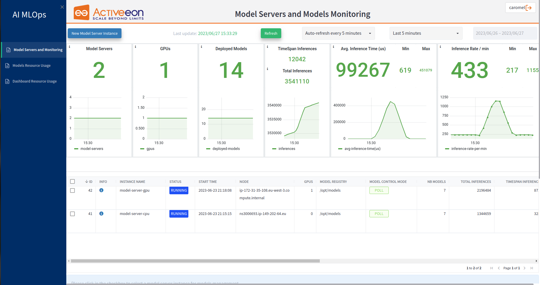
6.1. Model Servers and Monitoring
The Model Servers Monitoring tab focuses on overseeing the health and performance of the model servers or serving infrastructure. It is divided into two main parts.
In the first part, there are 6 main widgets providing general information about the model servers. These widgets offer valuable insights into the overall performance and usage of the serving infrastructure. Here are the widgets included in this tab:
-
Model Servers: This widget displays the number of currently running model servers. It provides a quick overview of the active instances responsible for serving machine learning models.
-
GPUs: This widget shows the number of running GPUs. It indicates the availability and utilization of GPU resources within the model servers, which is particularly relevant for GPU-accelerated machine learning workloads.
-
Deployed Models: This widget provides the total count of deployed models. It offers a summary of the number of machine learning models that have been successfully deployed and are currently running on the model servers.
-
TimeSpan Inferences and Total Inferences: These widgets track the number of inferences performed within a specific timespan and the total number of inferences overall. They give insights into the workload and usage patterns of the deployed models, allowing teams to assess the level of usage and demand for the served models.
-
Average Inference Time: This widget displays the average time taken for an inference to be processed. It provides an indication of the computational efficiency and latency of the model servers in generating predictions or inferences. Additionally, the minimum and maximum inference times help identify the performance variations.
-
Average Inference Rate: This widget shows the average rate at which inferences are processed, indicating the throughput or number of inferences handled per unit of time (per minute). The minimum and maximum inference rates provide insights into the server’s capacity and ability to handle varying workloads.
In the second part of the Model Servers Monitoring tab, there is a table listing the model servers along with their respective specific characteristics. The table provides detailed information about each model server instance. Here are the columns representing the characteristics of the model servers:
-
ID: This column displays the unique identifier assigned to each model server instance for easy reference and identification.
-
Info: The Info column presents relevant variables and their corresponding values used to launch the model server. It includes details such as the Docker Image utilized, GPU Enabled status, Endpoint ID, Node Source, and whether it is Proxyfied or not.
-
Logs: The Logs button provides access to detailed logs for model servers, allowing users to monitor and review the model server deployment, activity, and error messages.
-
Instance Name: This column specifies the name given to the model server instance, enabling users to easily identify and differentiate between different instances.
-
Status: The Status column indicates the current status of the model server instance. It provides important visibility into the current state of each model server instance, allowing users to quickly identify whether an instance is actively serving, has completed its task, or requires further attention due to issues encountered. It can take one of the following values:
-
Running: This status indicates that the model server instance is currently active and operational, ready to serve model predictions or inferences.
-
Finished: The "Finished" status indicates that the model server instance is no longer active and not serving predictions.
-
Finished with issues: The "Finished with issues" status indicates that the model server instance has encountered problems or issues during its operation. It suggests that the instance has completed its task, but there may have been complications or errors along the way that require attention or investigation.
-
-
Start Time: The Start Time column indicates the datetime when the model server instance was initiated.
-
Node: This column identifies the specific node or machine where the model server instance is running, providing insights into the underlying infrastructure allocation.
-
GPUs: The GPUs column displays the number of GPUs utilized by the corresponding model server instance. It highlights the GPU resource allocation for each instance, particularly useful for GPU-accelerated workloads.
-
Model Registry: This column indicates the location or source where the deployed models are stored, facilitating easy access and retrieval.
-
Model Control Mode: The Model Control Mode column specifies the mode of model control for the server instance, which can be Poll or None: where all actions can be performed using this mode such as deploying, undeploying, activating or deactivating models, or Explicit: where the models can be activated and deactivated but can not be deployed or undeployed. Using the Model Control Mode all models are loaded from the Model Registry in which models that can not be loaded are marked as UNAVAILABLE.
-
Nb of models: This column shows the count of models deployed on the specific model server instance, providing an overview of the model quantity hosted on that instance.
-
Total Inferences: The Total Inferences column represents the total number of inferences performed on the model server instance since its start.
-
TimeSpan Inferences: This column displays the number of inferences performed on the model server instance within a specified timespan.
-
Average Inference Time: The Average Inference Time column indicates the average duration taken by the model server instance to process an inference.
-
Min Inference Time: This column represents the minimum time taken for an inference on the model server instance.
-
Max Inference Time: The Max Inference Time column displays the maximum time taken for an inference on the model server instance.
-
Inference Rate: This column presents the rate or frequency at which inferences are processed by the model server instance, indicating the throughput or performance of the server.
-
Min Inference Rate: The Min Inference Rate column shows the lowest inference rate observed on the model server instance.
-
Max Inference Rate: This column represents the highest inference rate observed on the model server instance.
-
Actions: The Actions column contains buttons that allow users to interact with the model server instance. It includes options such as (1) Deploy a new Model on a running instance, (2) Stop a running model server instance, or (3) Re-Submit a stopped model server instance.
At the top of this tab, there is a "New Model Server Instance" button that allows users to launch a new model server. When clicked, a window will open, presenting variables that need to be specified by the user. There are two types of variables: General or Advanced. The Table below displays all the variables used to start a new model server.
Variable name |
Description |
Type |
Workflow variables |
||
|
Instance name of the new model server. |
String (default=Empty) [General]. |
|
If True, container will run with NVIDIA GPU support. |
Boolean (default=False) [General]. |
|
Path to the model repository. |
String (default="/opt/models") [General]. |
|
The model control mode determines how changes to the model repository are handled by the model server. |
List [none, explicit, poll] (default="explicit") [General]. |
|
If not empty, the workflow tasks will be run only on nodes belonging to the specified node source. |
List [Default, LocalNodes] (default=Empty) [Advanced]. |
|
If not empty, the workflow tasks will be run only on nodes that contains the specified token. |
List [model-server-xxx] (default=Empty) [Advanced]. |
|
Parameters given to the native scheduler (SLURM, LSF, etc) while requesting a ProActive node used to deploy the workflow tasks. |
String (default=Empty) [Advanced]. |
|
Docker image used to start the model server. |
String (default="nvcr.io/nvidia/tritonserver:22.10-py3") [Advanced]. |
In the model servers table, when a model server is selected, it shows another subtable that lists all the models stored in the model registry of that specific model server.
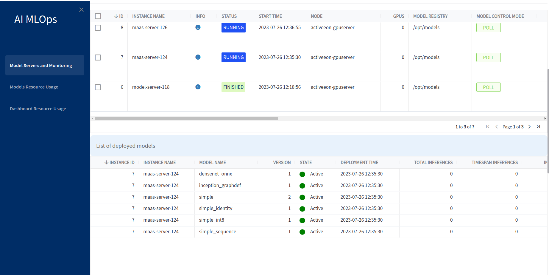
This subtable provides additional information about each model. Here are the columns characterizing each model:
-
Server Name: The Server Name column displays the name of the model server where the model is deployed, providing a clear association between the model and its corresponding server.
-
Model Name: This column represents the name or identifier of the model deployed on the model server, allowing for easy identification and differentiation between different models.
-
Version: The Version column indicates the version of the model deployed. It is particularly relevant when a model has multiple deployed versions. Model versioning enables reproducibility and traceability, facilitates performance monitoring and evaluation of different model versions, supports experimentation and iterative development, provides a safety net for rollbacks and recovery, and enhances collaboration and teamwork among data scientists.
-
State: The State column specifies the current state of the model, which can be Active or Inactive. It indicates whether the model is actively serving predictions or has been deactivated.
-
Deployment Time: The Deployment Time column denotes the timestamp or date when the model was deployed on the model server, providing visibility into the model’s deployment history.
-
Total Inferences: This column represents the total number of inferences performed by the model since its deployment on the model server.
-
TimeSpan Inferences The TimeSpan Inferences column displays the number of inferences performed by the model within a specific timespan, allowing for tracking and monitoring of recent model activity.
-
Inference Time: The Inference Time column indicates the average duration taken by the model to process an inference.
-
Min Inference Time: This column represents the minimum time taken for an inference by the model.
-
Max Inference Time: The Max Inference Time column displays the maximum time taken for an inference by the model.
-
Inference Rate: This column presents the rate or frequency at which inferences are processed by the model, indicating the throughput or performance of the model.
-
Min Inference Rate: The Min Inference Rate column shows the lowest inference rate observed for the model.
-
Max Inference Rate: This column represents the highest inference rate observed for the model.
-
Actions: The Actions column contains buttons that allow users to interact with the model. The available actions depend on the Model Control Mode of the corresponding model server. For model servers with Model Control Mode as Poll or None, the "Undeploy" button is available to remove the model from the server. For model servers with Model Control Mode as Poll, None, or Explicit, the "Activate" and "Deactivate" buttons are available to control the state of the model.
This tab and the other two tabs include a "Refresh" button, which, when clicked, refreshes the page and displays the last update datetime.
Additionally, all tabs offer an autorefresh feature that allows users to specify the time period for automatic refreshing. Users can choose from a list of predefined time periods, such as 15 seconds, 30 seconds, 5 minutes, 15 minutes, 30 minutes, 1 hour, etc., to determine how frequently the page should be refreshed automatically.
All the values displayed in the widgets and tables are calculated based on a selected time window. The time window can be chosen from a list of predefined options located at the top of the page, such as "Last 15 minutes," "Last 30 minutes," "Last 1 hour," "Last 24 hours," "Yesterday," "This month," "Previous month," and more. Alternatively, the user can select "Use Calendar," which activates a calendar feature. By choosing this option, the user can manually select the desired "From" and "To" dates, allowing for a custom time window selection.
6.2. Models Resource Usage
The second tab of the MLOps monitoring dashboard is dedicated to the Models Resource Usage, providing users with valuable insights into the CPU and GPU resource utilization. This tab is thoughtfully divided into two main parts to ensure a comprehensive understanding of the system’s resource consumption.
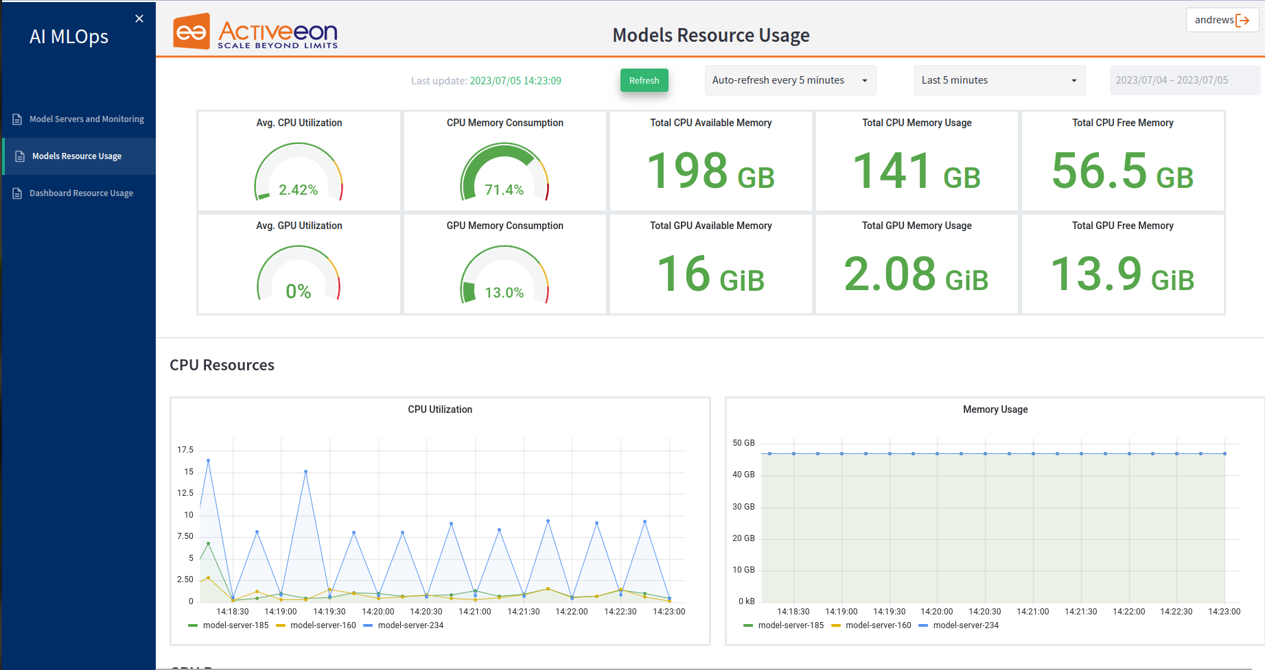
The first part features ten main widgets that offer users a wealth of general information about the CPU and GPU usage. These widgets provide real-time metrics, such as average CPU and GPU utilization, memory consumption, etc. By presenting this data in a visually appealing and easily comprehensible format, users can efficiently monitor and evaluate the overall resource consumption of their system. Whether it’s tracking performance trends or identifying potential bottlenecks, these widgets empower users to make informed decisions and optimize their resources effectively.
-
Avg. CPU Utilization and Avg. GPU Utilization: These widgets provide users with valuable insights into the average CPU and GPU utilization across all model servers. By calculating and displaying the average utilization percentages, users can quickly evaluate the overall resource usage of their model servers. These metrics allows users to gauge the overall CPU and GPU load and monitor any potential spikes or fluctuations in resource usage.
-
CPU Memory Consumption and GPU Memory Consumption: These widgets provide users with insights into the memory usage of both the CPU and GPU across all model servers allowing users to monitor the memory consumption patterns and identify any potential memory-related issues. These information are crucial for ensuring efficient memory allocation and optimizing the performance of the model servers.
-
Total CPU Available Memory and Total GPU Available Memory: These widgets present the overall amount of memory that is available for CPU and GPU usage across all model servers. They provide users with a numerical value in gigabytes (GB), indicating the total amount of memory that can be allocated to CPU tasks. These information allow users to understand the total capacity of CPU and GPU memory and make informed decisions regarding memory allocation for their models servers.
-
Total CPU Memory Usage and Total GPU Memory Usage: These widgets display the memory consumption of the CPU and GPU resources across all model servers. It presents users with information about the total amount of memory being used by the CPU, typically measured in gigabytes (GB). These metrics allow users to monitor the overall memory usage of the CPU and GPU resources and identify any potential memory-related issues or constraints.
-
Total CPU Free Memory and Total GPU Free Memory: These widgets present the amount of free memory available for CPU and GPU usage across all model servers. It would display a numerical value in gigabytes (GB). These information help users understand the remaining memory capacity that can be allocated to CPU and GPU tasks.
In the second part of the Model Resources Usage tab, there are several graphs that display time series data for each model server. These graphs provide users with detailed information about various metrics related to CPU and GPU utilization, memory usage, and power consumption. The first two graphs are related to CPU Resources and the rest of the graphs are related to GPU Resources:
-
CPU Utilization: This graph illustrates the CPU utilization over time for each model server. It presents the percentage of CPU resources being utilized by the respective servers, allowing users to analyze trends and identify periods of high or low CPU usage.
-
Memory Usage: This graph showcases the memory usage over time for each model server. It provides insights into the amount of memory being utilized by the servers, helping users monitor memory consumption patterns and identify any potential memory-related issues.
-
GPU Utilization This graph displays the GPU utilization over time for each model server. It shows the percentage of GPU resources being utilized by the servers, enabling users to track GPU usage trends and optimize resource allocation for GPU-intensive tasks.
-
Avg. GPU Utilization per Model Server: This graph presents the average GPU utilization per model server over time. It provides a comparative view of GPU utilization across different servers, allowing users to identify variations and patterns in resource usage.
-
GPU Used Memory: This graph visualizes the GPU memory usage over time for each model server. It illustrates the amount of GPU memory being actively used by the servers, aiding in monitoring memory consumption and optimizing GPU resource allocation.
-
GPU Free Memory: This graph shows the GPU free memory over time for each model server. It provides information about the available free memory on the GPUs, helping users track memory availability and ensure optimal memory usage.
-
GPU Power Usage (Watts): This graph displays the power usage of the GPUs over time for each model server. It shows the power consumption in watts, enabling users to monitor the energy usage of the GPUs and evaluate their power requirements.
6.3. Dashboard Resource Usage
The third tab in this dashboard is dedicated to "Dashboard Resource Usage" providing information about the resource consumption of the entire system, it focuses on monitoring the resources utilized by the MLOps infrastructure as a whole. This tab is divided into two main parts:
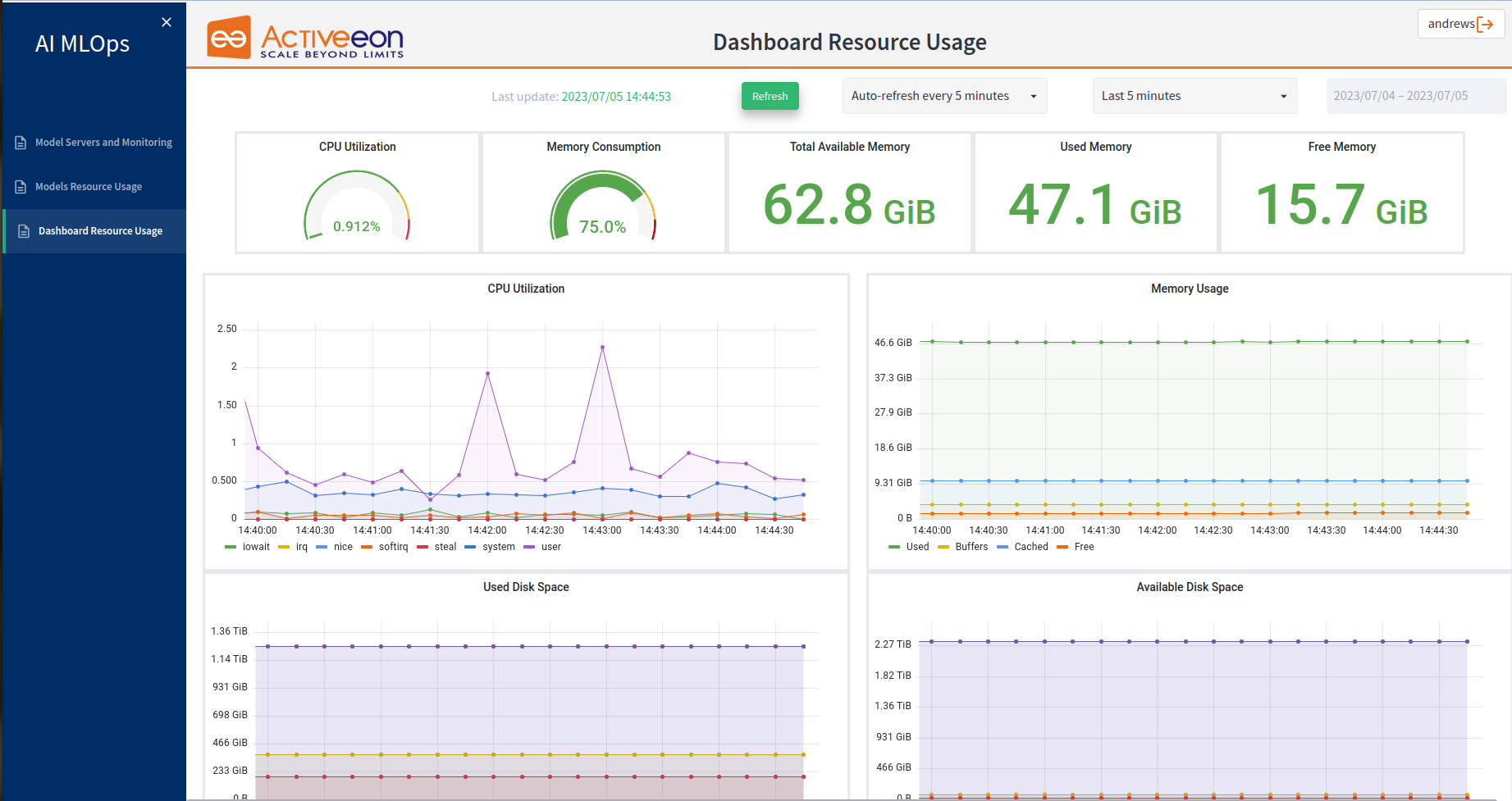
The first part focuses on providing information about the overall system. This part includes five main metrics:
-
CPU Utilization: This metric indicates the overall CPU utilization of the system. It provides information on the average or current CPU usage across all components of the MLOps infrastructure. Monitoring CPU utilization helps users assess the system’s workload and identify any potential performance issues or bottlenecks.
-
Memory Consumption: This metric reflects the total memory consumption of the system. It provides insights into the amount of memory being used by the MLOps infrastructure as a whole. Monitoring memory consumption helps users ensure sufficient memory resources are available and identify any excessive memory usage that may impact system performance.
-
Total Available Memory: This metric represents the total amount of memory available in the system. It provides an understanding of the overall memory capacity that can be allocated to various processes and applications within the MLOps infrastructure.
-
Used Memory: This metric indicates the total amount of memory currently in use by the system. It helps users assess the memory usage and understand how much memory is actively being utilized by processes and applications.
-
Free Memory: This metric reflects the amount of memory that is currently unoccupied and available for use. It helps users determine the remaining memory capacity in the system and ensure that sufficient free memory is available for optimal performance.
In the second part of the "Dashboard Resource Usage" tab, there are time series graphs that provide insights into various metrics related to CPU utilization, memory usage, disk memory, and network traffic. The specific graphs in this section include:
-
CPU Utilization:
-
iowait: indicates the percentage of time the CPU is idle but waiting for I/O operations.
-
irq: displays the CPU utilization due to hardware interrupts.
-
nice: represents the CPU utilization by processes with a user-defined priority.
-
softirq: shows the CPU utilization due to software interrupts.
-
steal: indicates the CPU utilization stolen by other virtual machines in a virtualized environment.
-
system: reflects the CPU utilization by the system/kernel processes.
-
user: represents the CPU utilization by user processes.
-
-
Memory Usage:
-
Used: displays the memory usage in use by the system.
-
Buffers: represents the memory used for buffering data from disk.
-
Cached: shows the memory used for caching data from disk.
-
Free: indicates the amount of free memory available in the system.
-
-
Used Disk Memory:
-
Graphs for specific files or directories, such as "/etc/timezone," "/usr/share/zoneinfo/Etc/UTC," "/etc/hostname," "/etc/hosts," "/etc/resolv.conf," "/etc/prometheus," "/opt/dashboard," and "/opt/grafana/conf." These graphs provide information about the disk memory usage for each specific file or directory.
-
-
Available Disk Space:
-
Graphs for specific files or directories, such as "/etc/timezone," "/usr/share/zoneinfo/Etc/UTC," "/etc/hostname," "/etc/hosts," "/etc/resolv.conf," "/etc/prometheus," "/opt/dashboard," and "/opt/grafana/conf." These graphs indicate the available disk space for each specific file or directory.
-
-
Network Traffic:
-
eth0 receive: displays the network traffic received on the eth0 network interface.
-
lo receive: represents the network traffic received on the loopback interface.
-
eth0 transmit: shows the network traffic transmitted on the eth0 network interface.
-
lo transmit: indicates the network traffic transmitted on the loopback interface.
-
6.4. Drift Notification
The Drift Notification tab enables users to create and manage drift monitoring instances, categorized into operational and data drift detection. This feature allows users to detect changes in the deployed models' performance due to shifts in either the input data distribution (data drift) or operational metrics (operational drift). By configuring drift notifications, users can receive alerts and take proactive measures to maintain the model’s accuracy and reliability, ensuring both data integrity and operational performance are preserved.
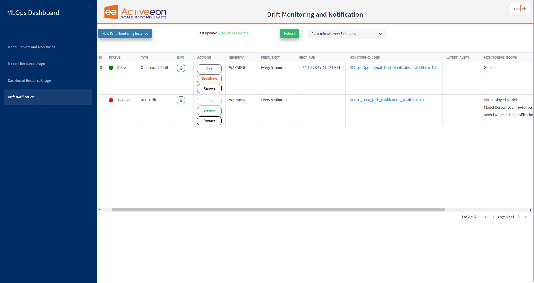
This page includes a table listing all the drift monitoring instances. Each column in the table provides specific information about the drift monitoring instance.
-
ID: Indicates the ID of the drift monitoring instance.
-
STATUS: Indicates the current status of the drift monitoring instance, such as Active or Inactive. It helps users quickly identify which instances are currently operational.
-
TYPE: Specifies whether the monitoring instance is set to detect data drift (changes in input data distribution) or operational drift (shifts in model performance metrics).
-
INFO: Displays the selected configuration values and settings for the drift monitoring instance.
-
ACTIONS: Provides a set of actionable buttons that allow users to manage the drift monitoring instance. Actions include Activate, Deactivate and Remove buttons.
-
SEVERITY: Displays the severity level of detected drift, such as INFO, WARNING, ERROR or CRITICAL. This helps prioritize which drift instances need immediate attention based on their potential impact on model performance.
-
FREQUENCY: Specifies how often the drift monitoring is performed. This indicates the regularity with which the monitoring instance checks for data drift.
-
NEXT_RUN: Indicates the scheduled time for the next execution of the drift monitoring instance to detect potential drift.
-
MONITORING_JOBS: Views all the job instances related to the corresponding drift monitoring instance in the ProActive Workflow Execution.
-
LATEST_ALERT: Displays the time when the most recent alert was sent for the drift monitoring instance.
-
MONITORING_SCOPE: Defines the scope of the monitoring instance, indicating whether it is Global, Per Model Server, or Per Deployed Model. This helps users understand the level at which drift monitoring is being applied, whether across all model servers, specific model servers, or individual deployed models.
-
TIME_FRAME: Defines the time period over which the drift is assessed which targets a specific historical period for analysis. It provides context for the drift analysis and trends over time.
-
METRIC: Specifies the metric used to measure drift, such as statistical tests or performance measures.
At the top of this page, there is a "New Drift Monitoring Instance" button that allows users to create a new monitoring instance. When clicked, a window will open, presenting variables that need to be specified by the user.
Variable name |
Description |
Type |
Workflow variables |
||
|
Type of the drift detection method to be used. |
List [Operational Drift Detection, Data Drift Detection] |
|
Monitoring scope for the drift notification. |
List [Global, Per Model Server, Per Deployed Model] (default="Global"). |
|
ID of the model server to be monitored. |
List [model-server-xxx] (default=model-server-xxx). |
|
Name of the deployed model to be monitored. |
List [model-name] (default=model-name). |
|
The temporal scope of the selected drift detection algorithm targets a specific historical period for analysis. |
List [Last xx minutes/hours/days] (default="Last 5 minutes"). |
|
The threshold for the number of drift occurences that trigger an alert. |
Integer (default=0) |
|
List of available metrics for the drift monitoring. |
List [avg_inference_time_ms, inference_rate_per_min ] (default="avg_inference_time_ms"). |
|
Name of the data drift detector to be used. |
List [Interval Threshold based, Threshold based, Statistical Threshold, HDDM_W, Page-Hinkley] (default=HDDM_W). |
|
Appears when choosing HDDM_W. It indicates the significance level required to declare a drift, influencing the algorithm’s sensitivity to changes in the data stream. |
Float (default=0.001). |
|
Appears when choosing HDDM_W. It Indicates significance level at which the algorithm issues a warning for potential drift. |
Float (default=0.005). |
|
Appears when choosing Interval Threshold based. Minimum cutoff value of the interval threshold. |
Float (default=0.0). |
|
Appears when choosing Interval Threshold based. Maximum cutoff value of the interval threshold. |
Float (default=0.01). |
|
Appears when choosing Threshold based . It is used to determine whether a value meets a specified threshold. |
List [less than, less than or equal to, equal to, greater than or equal to, greater than] (default=greater than). |
|
Appears when choosing Threshold based. Metric value used as a threshold value for comparison. |
Float (default=0.0). |
|
Appears when choosing Statistical Threshold. The number of standard deviations to use as the cutoff. |
Integer (default=2). |
|
Appears when choosing Page-Hinkley. Minimum number of instances before detecting change. |
Integer (default=30). |
|
Appears when choosing Page-Hinkley. Magnitude of change that will cause a signal. |
Float (default=0.005). |
|
Appears when choosing Page-Hinkley. Threshold for the Page-Hinkley test. |
Integer (default=50). |
|
Appears when choosing Page-Hinkley. Forgetting factor, it determines the weight given to newer data. |
Integer (default=50). |
|
The severity level for the notification. |
List [INFO, WARNING, ERROR, CRITICAL] (default="WARNING"). |
|
The timezone which indicates the geographical region of the user. |
List [timezone] (default="Europe/Paris"). |
|
Name of the channel to which the notification will be sent. |
String (default="mlops-dashboard"). |
|
Time frequency for scheduling drift analysis tasks. |
Integer (default=5). |
|
The time unit for the frequency used in drift analysis. |
List[minutes, hours, days] (default="minutes"). |
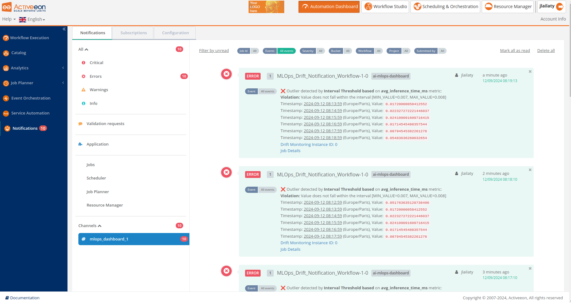
In case a drift in the input data occurs, a notification is sent to the dedicated channel specified in the NOTIFICATION_CHANNEL variable. This ensures that users are promptly informed about any significant changes in data distribution that may affect model performance. Here is an example of a drift notification from the ProActive Notification Portal:
7. AutoFeat
The performance of a machine learning model depends not only on the model and the hyper-parameters but also on how we process and feed different types of variables to the model.
Before starting the modelling phase, it is required to perform various tasks for data preparation. Encoding categorical data is one of the most crucial tasks. In real life, data commonly come with categorical string values and most of the machine learning models perform mathematical operations. However, the harsh truth is that mathematics is totally dependent on numbers. As a matter of fact, we can say that most of the machine learning models only accept numerical variables (generally floats or integers) and not strings. Then, preprocessing and encoding the categorical variables become a crucial step to convert these variables into numbers that can help in predicting the results in a machine learning task.
AutoFeat provides a complete solution to assist data scientists to encode successfully their categorical data.
In real-world problems, most of the time we require choosing one encoding method for the proper working of the model. Working with different encoders can influence the results of the model.
AutoFeat currently supports the following encoding methods:
-
Label: converts each value in a categorical feature into an integer value between 0 and n-1, where n is the number of distinct categories of the variable.
-
Binary: stores categories as binary bitstrings.
-
OneHot: creates a new feature for each category in the categorical variable and replaces it with either 1 (presence of the feature) or 0 (absence of the feature). The number of the new features depends on the number of categories in the categorical variable.
-
Dummy: transforms the categorical variable into a set of binary variables (also known as dummy variables). The dummy encoding is a small improvement over the one-hot-encoding, such it uses n-1 features to represent n categories.
-
BaseN: encodes the categories into arrays of their base-n representation. A base of 1 is equivalent to one-hot encoding and a base of 2 is equivalent to binary encoding.
-
Target: replaces a categorical value with the mean of the target variable.
-
Hash: maps each category to an integer within a pre-determined range n_components. n_components is the number of dimensions, in other words, the number of bits to use to represent the feature. We use 8 bits by default.
| The most of these methods are implemented using the python Category Encoders library. Examples can be found in the Category Encoders Examples notebook . |
As we already mentioned, the performance of ML algorithms depends on how categorical variables are encoded. The results produced by the model vary depending on the used encoding technique. Thus, the hardest part of categorical encoding can sometimes be finding the right categorical encoding method.
There are numerous research papers and studies dedicated to the analysis of the performance of categorical encoding approaches applied to different datasets. Based on the common factors shared by the datasets using the same encoding method, we have implemented an algorithm for finding the best suited method for your data.
To access the AutoFeat page, please follow the steps below:
-
Open the Studio Portal.
-
Create a new workflow.
-
Drag and drop the
Import_Data_And_Automate_Feature_Engineeringtask from theai-machine-learningbucket in the ProActive AI Orchestration. -
Click on the task and click
General Parametersin the left to change the default parameters of this task.
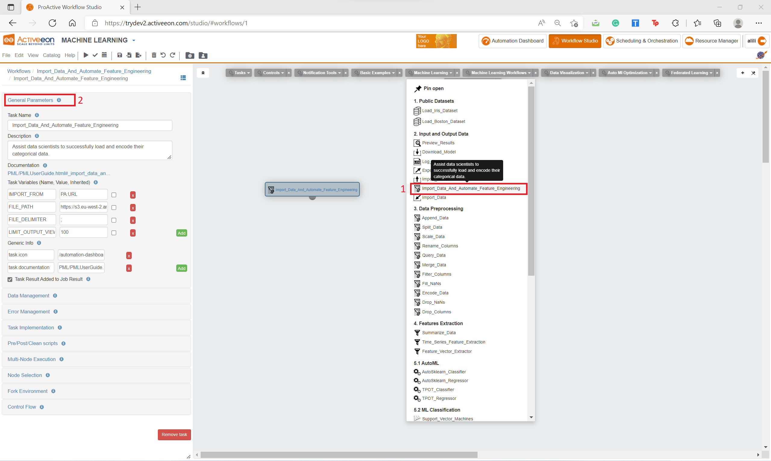
-
Put in FILE_PATH variable the S3 link to upload your dataset.
-
Set the other parameters according to your dataset format.
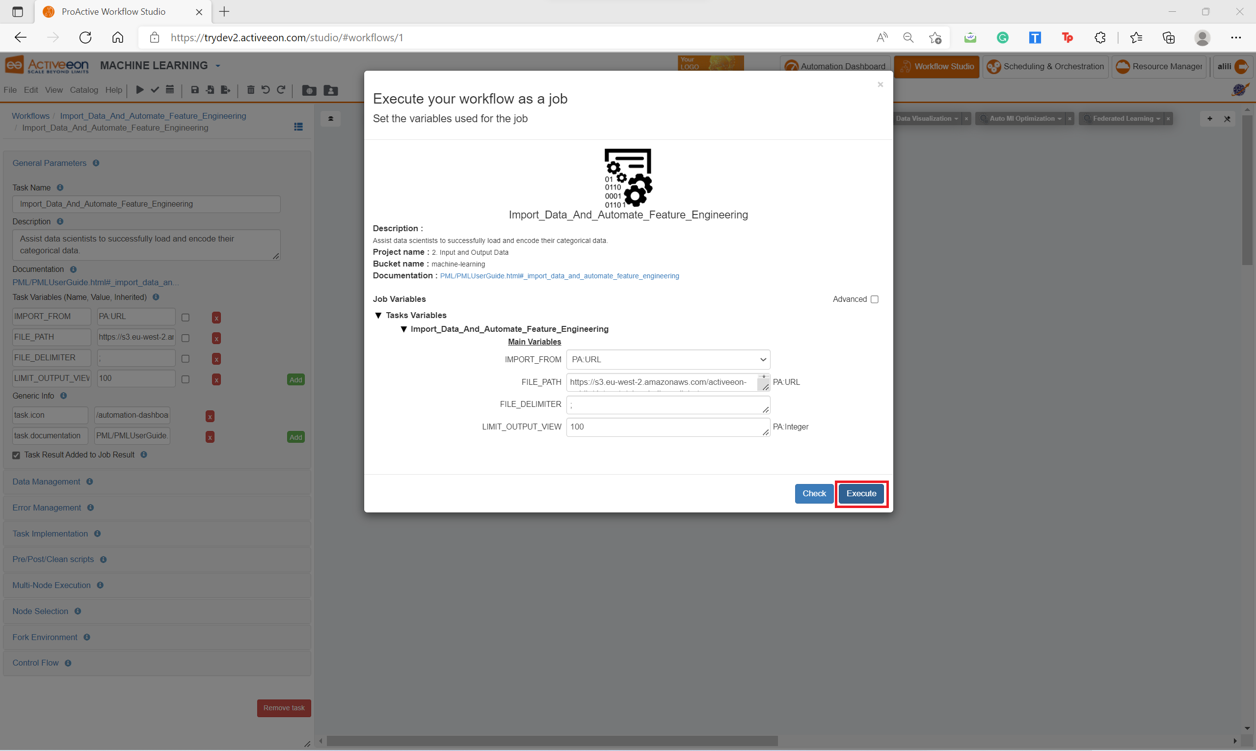
-
Click on the Execute button to run the workflow and start AutoFeat.
To get more information about the parameters of the service, please check the section Import_Data_And_Automate_Feature_Engineering.
-
Open the Workflow Execution Portal.
-
You can now access the AutoFeat Page by clicking on the endpoint
AutoFeatas shown in the image below.
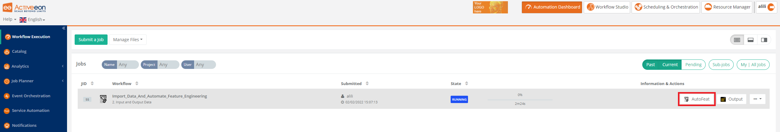
You will be redirected to AutoFeat page which initially contains three tabs that we describe in the following sections.
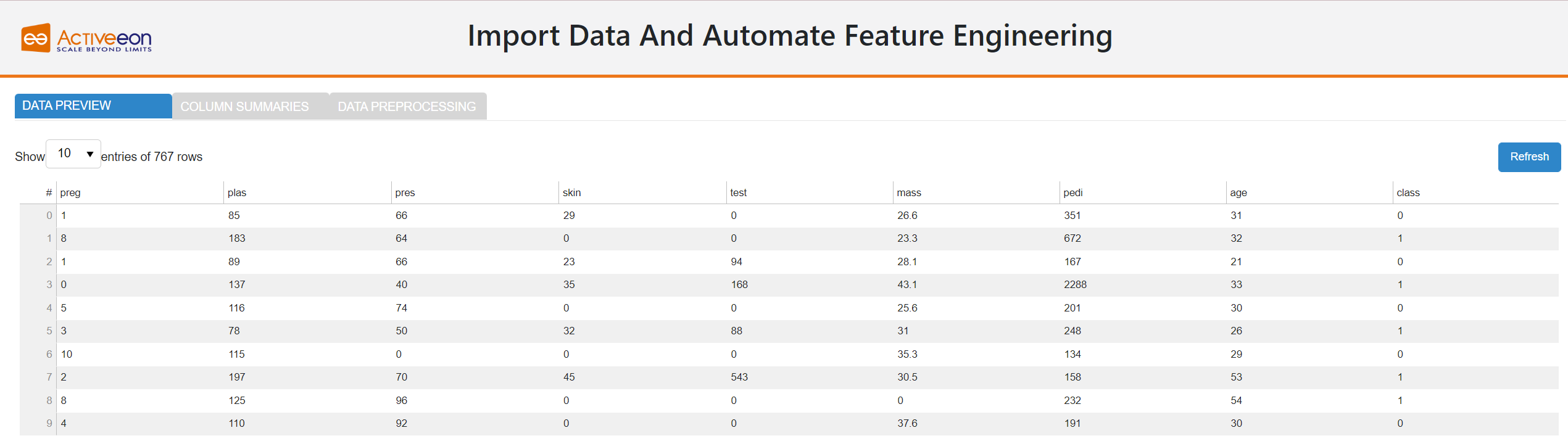
7.1. Data Preview
AutoFeat loads data from external sources. The dataset could be potentially very large. Initially, only the 10 first data rows are displayed.
The Refresh button enables users to see the last updates made on their data.
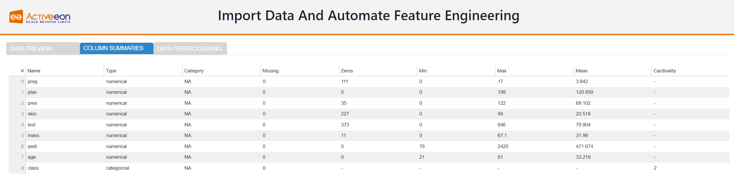
7.2. Column summaries
Whenever AutoFeat loads data from external sources, it also identifies the datatype of each column. AutoFeat does a great job at datatype recognition. Each decision can be overridden manually by the user, if required.
AutoFeat also creates some summary statistics for each column. A table is displaying the missing values, minimum, maximum, mean and zeros for each numerical feature, and the cardinality (category counts) for each categorical feature.
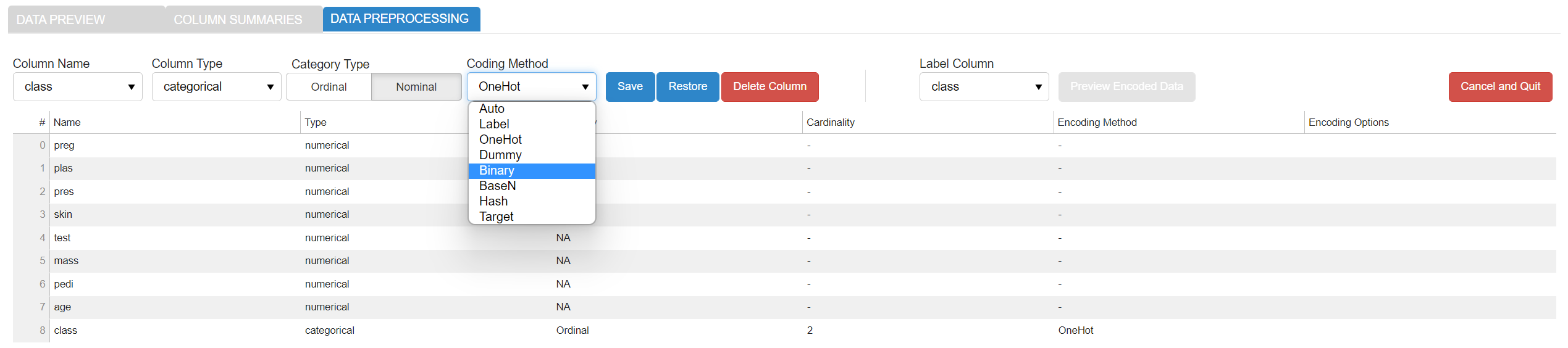
7.3. Data Preprocessing
A preview of the data is displayed in the Data Preprocessing as follows.
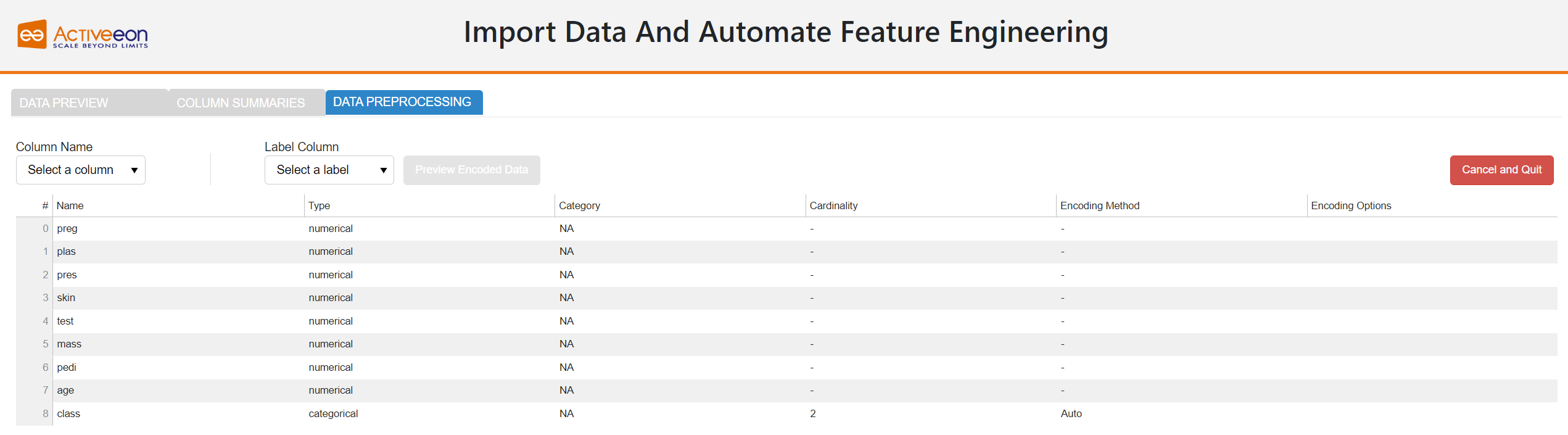
It is possible to change a column information. These changes can include:
-
Column Name: There should rarely be a reason to change the field name.
-
Column Type: AutoFeat automatically recognizes the data type, so the default settings typically do not need to be changed. There are two different data types; Categorical and Numerical.
-
Category Type: Categorical variables can be divided into two categories; Ordinal such the categories have an inherent order and Nominal if the categories do not have any inherent order.
-
Label Column: Only one column can be selected as the label column.
-
Coding Method: The encoding method used for converting the categorical data values into numerical values. The value is set to Auto by default. Thereafter, the best suited method for encoding the categorical feature is automatically identified. The data scientist still has the ability to override every decision and select another encoding method from the drop-down menu. Different methods are supported by AutoFeat such as Label, OneHot, Dummy, Binary, Base N, Hash and Target. Some of those methods require specifying additional encoding parameters. These parameters vary depending on the selected method (e.g., the base and the number of components for BaseN and Hash, respectively, and the target column for Target encoding method). Some of those values are set by default, if no values are specified by the user.
It is also possible to perform the following actions on the dataset:
-
Save, to save the last changes made on a column information.
-
Restore, to restore the original version of the dataset loaded from the external source.
-
Delete Column, to delete a column from the dataset.
-
Preview Encoded Data, to display the encoding results in a new tab.
-
Cancel and Quit, to discard any changes the user may have made and finish the workflow execution.
Once the encoding parameters are set, the user can proceed to display the encoded dataset by clicking on the Preview Encoded Data. He can also check and compare different encoding methods and/or parameters based on the obtained results.
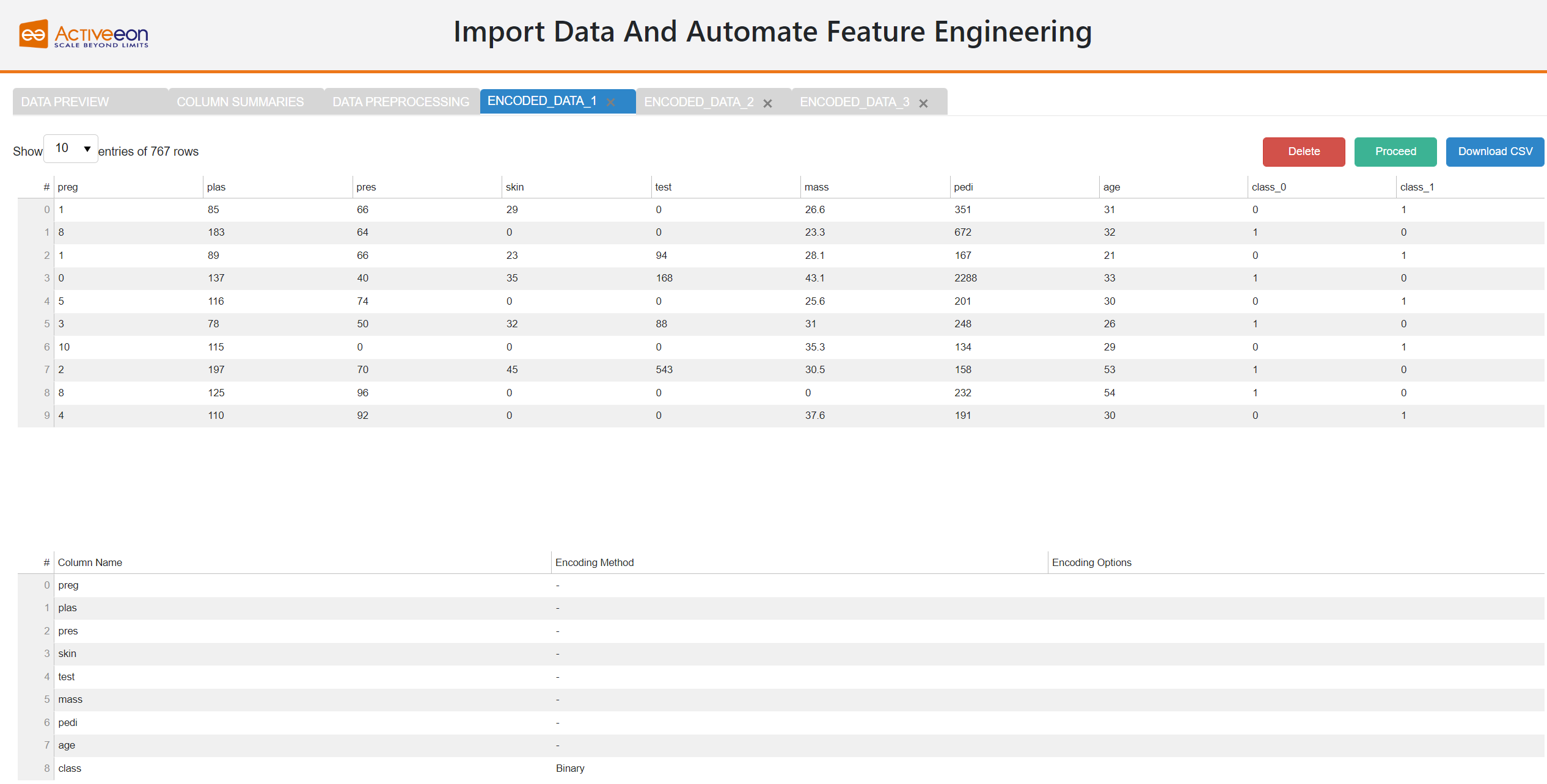
7.4. Encoded data
This page displays the data encoding results based on the selected parameters. At this stage, the user can validate the results by clicking on the button Proceed, or erase the encoded dataset by clicking on the button Delete.
The user can also download the results as a csv file by clicking on the Download button.
7.5. ML Pipeline Example
You can connect different tasks in a single workflow to get the full pipeline from data preprocessing to model training and deployment. Each task will propagate the acquired variables to its children tasks.
The following workflow example Vehicle_Type_Using_Model_Explainability uses the Import_Data_And_Automate_Feature_Engineering task to prepare the data. It is available on the machine_learning_workflows bucket.
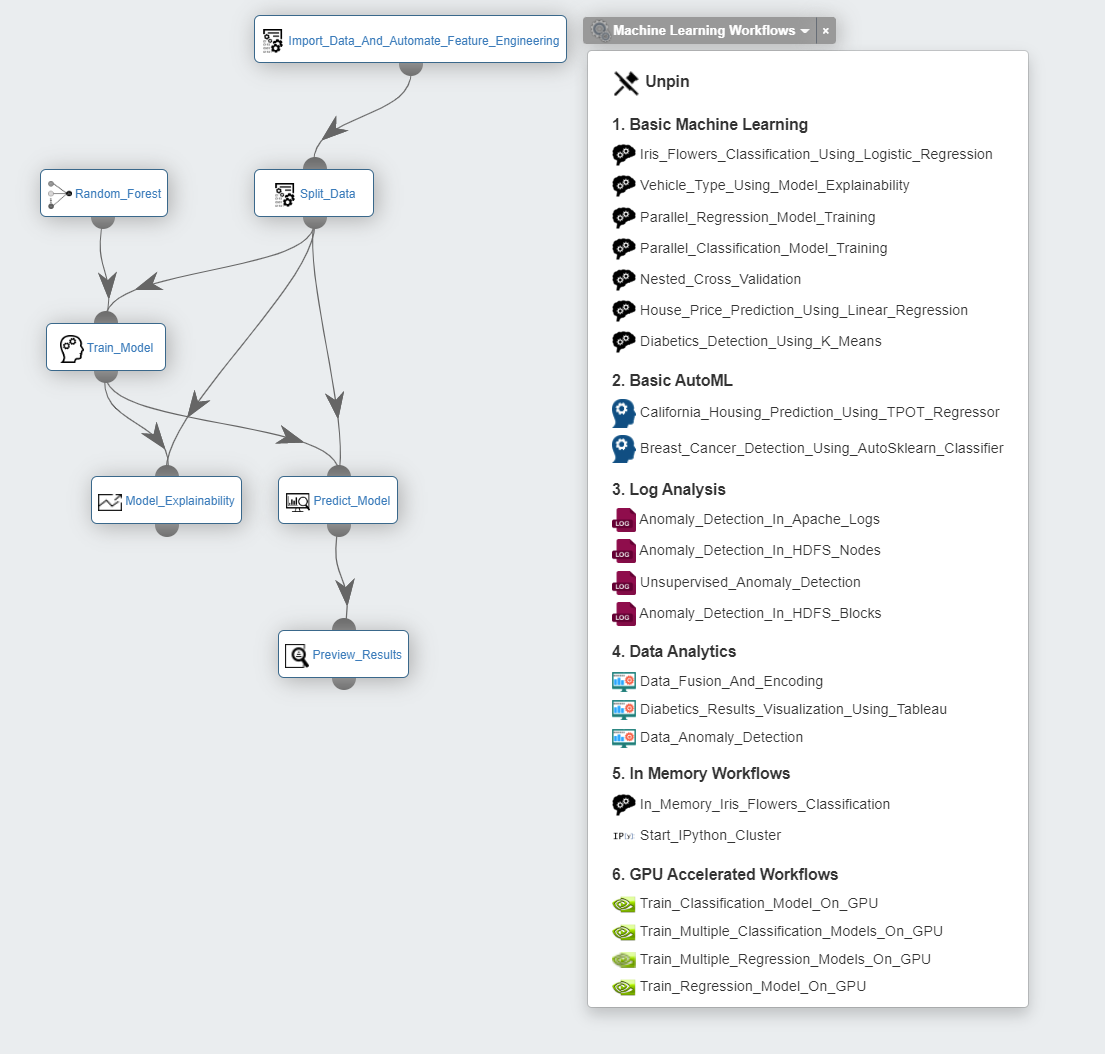
This workflow predicts vehicle type based on silhouette measurements, and apply ELI5 and Kernel Explainer to understand the model’s global behavior or specific predictions.
8. ProActive Analytics
The ProActive Analytics is a dashboard that provides an overview of executed workflows along with their input variables and results.
It offers several functionalities, including:
-
Advanced search by name, user, date, state, etc.
-
Execution metrics summary about durations, encountered issues, etc.
-
Charts to track variables and results evolution and correlation.
-
Data exportation in multiple formats for further use in analytics tools.
ProActive Analytics is very useful to compare metrics and charts of workflows that have common variables and results. For example, a ML algorithm might take different variables values and produce multiple results. It would be interesting to analyze the correlation and evolution of the algorithm results regarding the input variation (See also a similar example of AutoML). The following sections will show you some key features of the dashboard and how to use them for a better understanding of your job executions.
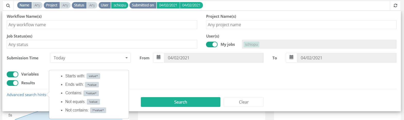
8.1. Job Analytics
Job Analytics Page includes a search window that allows users to search for jobs based on specific criteria (see screenshot below). The job search panel allows selecting multi-value filters for the following job parameters:
-
Workflow Name(s): Jobs can be filtered by workflow name. Selecting/Typing one or more workflow names is provided by a built-in
auto-completefeature that helps you search for workflows or buckets from the ProActive Catalog. -
Project Name(s): You can also filter by one or more project names. You just have to specify the project names for the jobs you would like to analyze.
-
Job Status: You can specify the state of jobs you are looking for. The possible job status are:
Pending,Running,Stalled,Paused,In_Error,Finished,Canceled,Failed, andKilled. For more information about job status, check the documentation here. Multiple values are accepted as well. -
User(s): This filter allows to either select only the jobs of the connected/current user or to specify a list of users that have executed the jobs. By default, the toggle filter is activated to select only the user jobs.
-
Submission Time: From the dropdown list, users can select a submission time frame (e.g., yesterday, last week, this month, etc.), or choose custom dates.
-
Variables and results: It is possible to choose whether to display or not the workflow’s variables and results. When deactivated, the charts related to variables and results evolution/correlation will not be displayed in the dashboard.
More advanced search options (highlighted in advanced search hints) could be used to provide filter values such as wildcards. For example, names that start with a specific string value are selected using value*. Other supported expressions are: *value for Ends with, *value* for Contains, !value for Not equals, and !*value* for Not contains.
Now you can hit the search button to request jobs from the scheduler database according to the provided filter values. The search bar at the top shows a summary of the active search filters.
8.1.1. Execution Metrics
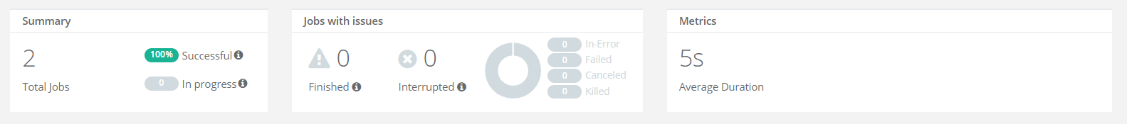
As shown in the screenshot below, Job Analytics Portal provides a summary of the most important job execution metrics. For instance, the dashboard shows:
-
A first panel that displays the number of total jobs that correspond to the search query. It also shows the ratio of successful jobs over the total number, and the number of jobs that are in progress and not yet finished. Please note that the number of in-progress jobs corresponds to the moment when the search query is executed and it is not automatically refreshed.
-
A second summary panel that displays the number of jobs with issues. We distinguish two types of issues: jobs that are finished but have encountered issues during their execution and interrupted jobs that did not finish their execution and were stopped due to diverse causes, such as insufficient resources, manual interruption, etc. Interrupted jobs include four status:
In-Error,Failed,Canceled, andKilled. -
The last metric gives an overview of the average duration of the selected jobs.
8.1.2. Job Charts
Job Analytics includes three types of charts:
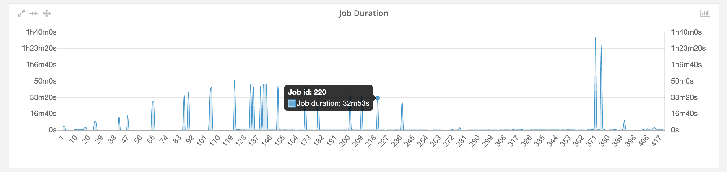
-
Job duration chart: This chart shows durations per job. The x-axis shows the job ID and the y-axis shows the job duration. Hovering over the lines will also display the same information as a tooltip (see screenshot below). Using the duration chart will eventually help the users to identify any abnormal performance behaviour among several workflow executions.
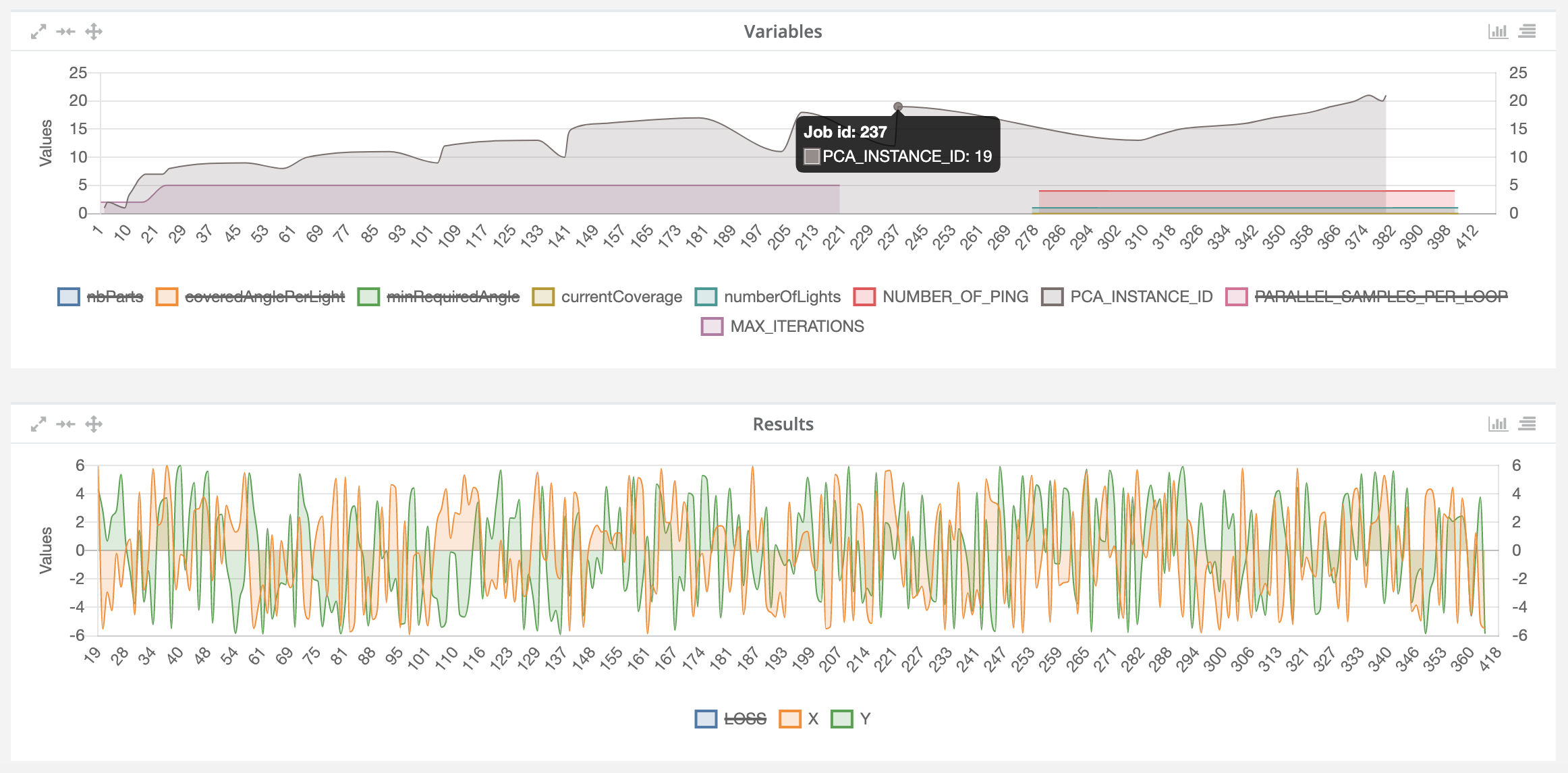
-
Job variables chart: This chart is intended to show all variable values of selected jobs. It represents the evolution chart for all numeric-only variables of the selected jobs. The chart provides the ability to hide or show specific input variables by clicking on the variable name in the legend, as shown in the figure below.
-
Job results chart: This chart is intended to show all result values of selected jobs. It represents the evolution chart for all numeric-only results of the selected jobs. The chart provides also the ability to hide or show specific results by clicking on the variable name in the legend, as shown in the figure below.
All charts provide some advanced features such as "maximize" and "enlarge" to better visualize the results, and "move" to customize the dashboard layout (see top left side of charts). All of them provide the hovering feature as previously described and two types of charts to display: line and bar charts. Switching from one to the other can be activated through a toggle button located at the top right of the chart. Same for show/hide variables and results.
8.1.3. Job Execution Table
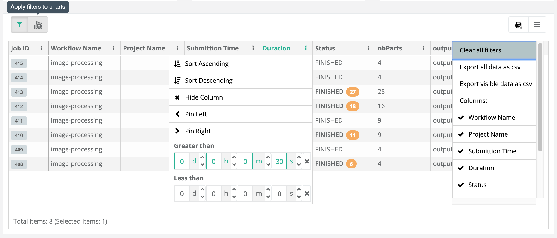
The last element of the Job Analytics dashboard shows a summary table that contains all job executions returned by the search query. It includes the job ID, status, duration, submission time, variables, results, etc. The jobs table provides many features:
-
Filtering: users can specify filter values for every column. For instance, the picture below applies a filter on the duration where we filter only jobs that last more than 30s. For string values, we can apply string-related filters such as Contains. For dates, a calendar is displayed to help users select the right date. Please note that variables and results types are not automatically detected. Therefore, users can choose either the Contains filter or the Greater than and Less than filters.
-
Sort, hide, pin left and right columns: allows users to easily handle and display data with respect to their needs.
-
Export the job data to CSV format: enables users to exploit and process job data using other analytics tools such as R, Matlab, BI tools, ML APIs, etc.
-
Clear and apply filters: When filters are applied, the displayed data is updated. Therefore, we provide a button (see apply filters to charts on the top left of the of the table screenshot) that allows synchronizing the charts with the filtered data in the table. Finally, it is possible to clear all filters. This will automatically deactivate the synchronization.
-
Link to scheduler jobs: data in the job ID column is linked to the job executions in the scheduler. For example, if users want to access to the logs of a failing job, they can click on the corresponding job ID to be redirected to the job location in the Scheduling Portal.
We note also that clicking on the issue types and charts described in the previous sections filters the table to show the corresponding jobs.
| It is important to notice that the dashboard layout and search preferences are saved in the browser cache so that users can have access to their last dashboard and search settings. |
9. ProActive Jupyter Kernel
The ActiveEon Jupyter Kernel adds a kernel backend to Jupyter. This kernel interfaces directly with the ProActive scheduler and constructs tasks and workflows to execute them on the fly.
With this interface, users can run their code locally and test it using a native python kernel, and by a simple switch to ProActive kernel, run it on remote public or private infrastructures without having to modify the code. See the example below:
9.1. Installation
9.1.1. Requirements
Python 2 or 3
9.1.2. Using PyPi
-
open a terminal
-
install the ProActive jupyter kernel with the following commands:
$ pip install proactive proactive-jupyter-kernel --upgrade
$ python -m proactive-jupyter-kernel.install
9.1.3. Using source code
-
open a terminal
-
clone the repository on your local machine:
$ git clone git@github.com:ow2-proactive/proactive-jupyter-kernel.git-
install the ProActive jupyter kernel with the following commands:
$ pip install proactive-jupyter-kernel/
$ python -m proactive-jupyter-kernel.install
9.2. Platform
You can use any jupyter platform. We recommend to use jupyter lab. To launch it from your terminal after having installed it:
$ jupyter labor in daemon mode:
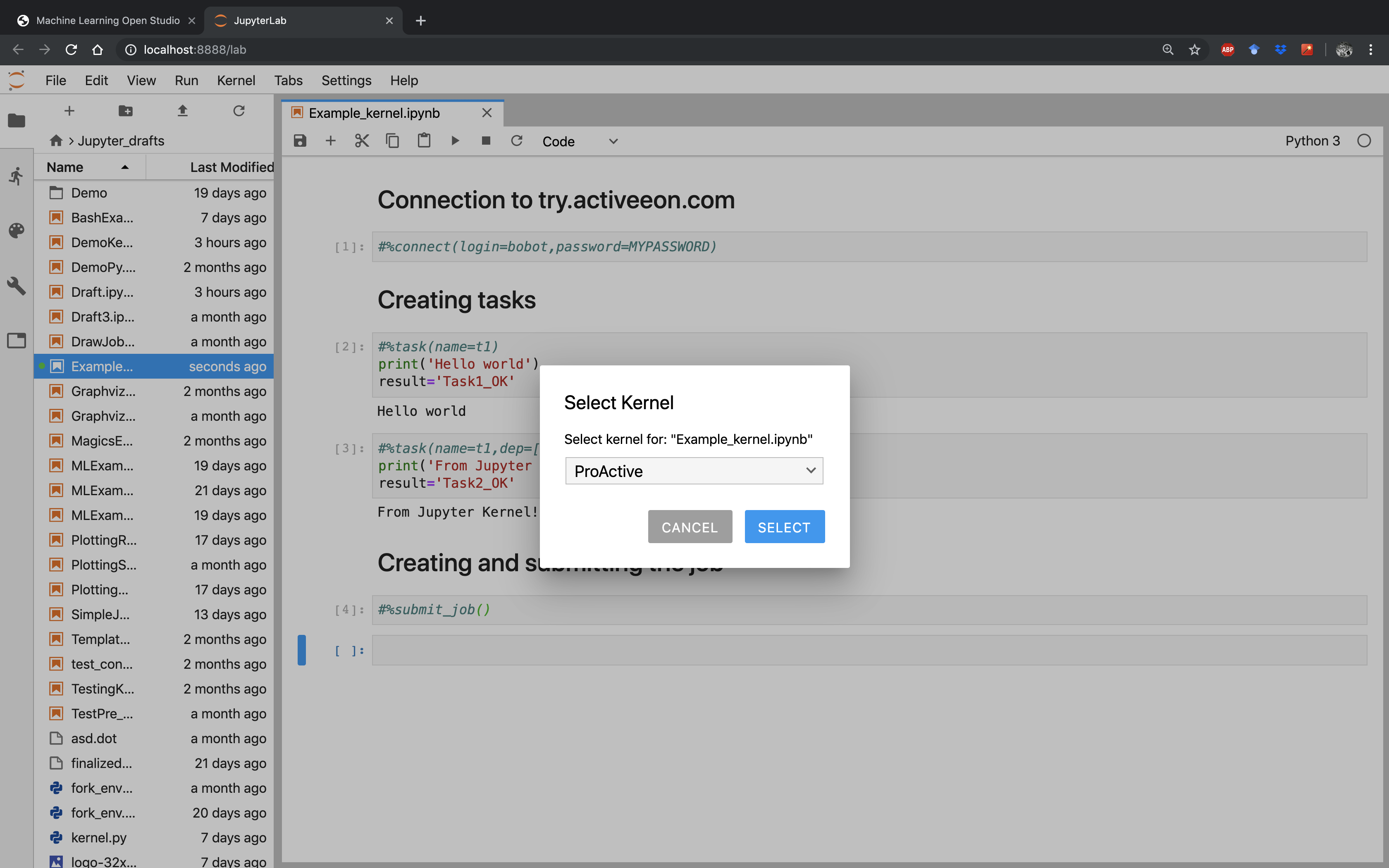
$ nohup jupyter lab &>/dev/null &When opened, click on the ProActive icon to open a notebook based on the ProActive kernel.
9.3. Help
As a quick start, we recommend the user to run the #%help() pragma using the following script:
#%help()This script gives a brief description of all the different pragmas that the ProActive Kernel provides.
To get a more detailed description of a needed pragma, the user can run the following script:
#%help(pragma=PRAGMA_NAME)9.4. Connection
9.4.1. Using connect()
If you are trying ProActive for the first time, sign up on the try platform.
Once you receive your login and password, connect to the trial platform using the #%connect() pragma:
#%connect(login=YOUR_LOGIN, password=YOUR_PASSWORD)To connect to another ProActive server host, use the later pragma this way:
#%connect(host=YOUR_HOST, [port=YOUR_PORT], login=YOUR_LOGIN, password=YOUR_PASSWORD)
Notice that the port parameter is optional. The default connexion port is 8080.
|
You can also connect to a distant server by providing its url in the following way:
#%connect(url=YOUR_SERVER_URL, login=YOUR_LOGIN, password=YOUR_PASSWORD)By providing the complete url of the server, users can eventually connect through the secure HTTPS protocol.
9.4.2. Using a configuration file
For automatic sign in, create a file named proactive_config.ini in your notebook working directory.
Fill your configuration file according to one of the following two formats:
-
By providing the server
hostandport:
[proactive_server]
host=YOUR_HOST
port=YOUR_PORT
[user]
login=YOUR_LOGIN
password=YOUR_PASSWORD-
By providing the server
url:
[proactive_server]
url=YOUR_SERVER_URL
[user]
login=YOUR_LOGIN
password=YOUR_PASSWORD
Save your changes and restart the ProActive kernel.
You can also force the current kernel to connect using any .ini config file through the #%connect() pragma:
#%connect(path=PATH_TO/YOUR_CONFIG_FILE.ini)(For more information about this format please check configParser)
9.5. Usage
9.5.1. Creating a Python task
To create a new task, use the pragma #%task() followed by the task implementation script written into a notebook
block code.
To use this pragma, a task name has to be provided at least. Example:
#%task(name=myTask)
print('Hello world')
General usage:
#%task(name=TASK_NAME, [language=SCRIPT_LANGUAGE], [dep=[TASK_NAME1,TASK_NAME2,...]], [generic_info=[(KEY1,VAL1), (KEY2,VALUE2),...]], [variables=[(VAR1,VAL1), (VAR2,VALUE2),...]], [export=[VAR_NAME1,VAR_NAME2,...]], [import=[VAR_NAME1,VAR_NAME2,...]], [path=IMPLEMENTATION_FILE_PATH])\n'Users can also provide more information about the task using the pragma’s options. In the following, we give more details about the possible options:
Language
The language parameter is needed when the task script is not written in native Python. If not provided, Python will be
selected as the default language.
The supported programming languages are:
-
Linux_Bash
-
Windows_Cmd
-
DockerCompose
-
Scalaw
-
Groovy
-
Javascript
-
Jython
-
Python
-
Ruby
-
Perl
-
PowerShell
-
R
Here is an example that shows a task implementation written in Linux_Bash:
#%task(name=myTask, language=Linux_Bash)
echo 'Hello, World!'
Dependencies
One of the most important notions in workflows is the dependencies between tasks. To specify this information, use the
dep parameter. Its value should be a list of all tasks on which the new task depends. Example:
#%task(name=myTask,dep=[parentTask1,parentTask2])
print('Hello world')
Variables
To specify task variables,
you should provide the variables parameter. Its value should be a list of tuples (key,value) that corresponds to
the names and adequate values of the corresponding task variables. Example:
#%task(name=myTask, variables=[(var1,value1),(var2,value2)])
print('Hello world')
Generic information
To specify the values of some advanced ProActive variables called
Generic Information, you should
provide the generic_info parameter. Its value should be a list of tuples (key,value) that corresponds to the names
and adequate values of the Generic Information. Example:
#%task(name=myTask, generic_info=[(var1,value1),(var2,value2)])
print('Hello world')
Export/import variables
The export and import parameters ensure variables propagation between the different tasks of a workflow.
If myTask1 variables var1 and var2 are needed in myTask2, both pragmas have to specify this information as
follows:
-
myTask1should include anexportparameter with a list of these variable names, -
myTask2should include animportparameter with a list including the same names.
Example:
myTask1 implementation block would be:
#%task(name=myTask1, export=[var1,var2])
var1 = "Hello"
var2 = "ActiveEon!"
and myTask2 implementation block would be:
#%task(name=myTask2, dep=[myTask1], import[var1,var2])
print(var1 + " from " + var2)
Implementation file
It is also possible to use an external implementation file to define the task implementation. To do so, the option path
should be used.
Example:
#%task(name=myTask,path=PATH_TO/IMPLEMENTATION_FILE.py)9.5.2. Importing libraries
The main difference between the ProActive and 'native language' kernels resides in the way the memory is accessed
during blocks execution. In a common native language kernel, the whole script code (all the notebook blocks) is
locally executed in the same shared memory space; whereas the ProActive kernel will execute each created task in an
independent process. In order to facilitate the transition from native language to ProActive kernels, we included the
pragma #%import(). This pragma gives the user the ability to add libraries that are common to all created tasks, and
thus relative distributed processes, that are implemented in the same native script language.
The import pragma is used as follows:
#%import([language=SCRIPT_LANGUAGE]).
Example:
#%import(language=Python)
import os
import pandas| If the language is not specified, Python is considered as default language. |
9.5.3. Adding a fork environment
To configure a fork environment for a task, use the #%fork_env() pragma. To do so, you have to provide the name of the
corresponding task and the fork environment implementation.
Example:
#%fork_env(name=TASK_NAME)
dockerImageName = 'activeeon/dlm3'
dockerRunCommand =  'docker run '
dockerParameters = '--rm '
paHomeHost = variables.get("PA_SCHEDULER_HOME")
paHomeContainer = variables.get("PA_SCHEDULER_HOME")
proActiveHomeVolume = '-v '+paHomeHost +':'+paHomeContainer+' '
workspaceHost = localspace
workspaceContainer = localspace
workspaceVolume = '-v '+localspace +':'+localspace+' '
containerWorkingDirectory = '-w '+workspaceContainer+' '
preJavaHomeCmd = dockerRunCommand + dockerParameters + proActiveHomeVolume + workspaceVolume + containerWorkingDirectory + dockerImageName
Or, you can provide the task name and the path of a .py file containing the fork environment code:
#%fork_env(name=TASK_NAME, path=PATH_TO/FORK_ENV_FILE.py)9.5.4. Adding a selection script
To add a selection script to a task, use the #%selection_script() pragma. To do so, you have to provide the name of
the corresponding task and the selection code implementation.
Example:
#%selection_script(name=TASK_NAME)
selected = True
Or, you can provide the task name and the path of a .py file containing the selection code:
#%selection_script(name=TASK_NAME, path=PATH_TO/SELECTION_CODE_FILE.py)9.5.5. Adding job fork environment and/or selection script
If the selection scripts and/or the fork environments are the same for all job tasks, we can add them just once using
the job_selection_script and/or the job_fork_env pragmas.
Usage:
For a job selection script, please use:
#%job_selection_script([language=SCRIPT_LANGUAGE], [path=./SELECTION_CODE_FILE.py], [force=on/off])For a job fork environment, use:
#%job_fork_env([language=SCRIPT_LANGUAGE], [path=./FORK_ENV_FILE.py], [force=on/off])The force parameter defines whether the pragma has to overwrite the task selection scripts or the fork environment
already set.
9.5.6. Adding pre and/or post scripts
Sometimes, specific scripts has to be executed before and/or after a particular task. To do that, the solution provides
pre_script and post_script pragmas.
To add a pre-script to a task, please use:
#%pre_script(name=TASK_NAME, language=SCRIPT_LANGUAGE, [path=./PRE_SCRIPT_FILE.py])To add a post-script to a task, use:
#%post_script(name=TASK_NAME, language=SCRIPT_LANGUAGE, [path=./POST_SCRIPT_FILE.py])9.5.7. Branch control
The branch control provides the ability to choose between two alternative task flows, with the possibility to merge back to a common one.
To add a branch control to the current workflow, four specific tasks and one control condition should be added in accordance with the following order:
-
a
branchtask, -
the related branching
conditionscript, -
an
iftask that should be executed if the result of theconditiontask iftrue, -
an
elsetask that should be executed if the result of theconditiontask iffalse, -
a
continuationtask that should be executed after theifor theelsetasks.
To add a branch task, you can rely on the following macro:
#%branch([name=TASK_NAME], [dep=[TASK_NAME1,TASK_NAME2,...]], [generic_info=[(KEY1,VAL1), (KEY2,VALUE2),...]], [language=SCRIPT_LANGUAGE], [path=./FORK_ENV_FILE.py])For the branching condition script, use:
#%condition()For an if task, please use:
#%if([name=TASK_NAME], [generic_info=[(KEY1,VAL1),(KEY2,VALUE2),...]], [language=SCRIPT_LANGUAGE], [path=./FORK_ENV_FILE.py])For an else task, use:
#%else([name=TASK_NAME], [generic_info=[(KEY1,VAL1),(KEY2,VALUE2),...]], [language=SCRIPT_LANGUAGE], [path=./FORK_ENV_FILE.py])And finally, for the continuation task:
#%continuation([name=TASK_NAME], [generic_info=[(KEY1,VAL1),(KEY2,VALUE2),...]], [language=SCRIPT_LANGUAGE], [path=./FORK_ENV_FILE.py])9.5.8. Loop control
The loop control provides the ability to repeat a set of tasks.
To add a loop control to the current workflow, two specific tasks and one control condition should be added in the following order:
-
a
starttask, -
the related looping
conditionscript, -
a
looptask.
For a start task, use:
#%start([name=TASK_NAME], [dep=[TASK_NAME1,TASK_NAME2,...]], [generic_info=[(KEY1,VAL1), (KEY2,VALUE2),...]], [language=SCRIPT_LANGUAGE], [path=./FORK_ENV_FILE.py])For the looping condition script, use:
#%condition()For a loop task, please use:
#%loop([name=TASK_NAME], [generic_info=[(KEY1,VAL1),(KEY2,VALUE2),...]], [language=SCRIPT_LANGUAGE], [path=./FORK_ENV_FILE.py])9.5.9. Replicate control
The replication allows executing multiple tasks in parallel when only one task is defined, and the number of tasks to run could change.
Through the ProActive Jupyter Kernel, users can add replicate controls in two main ways, a generic and a straight forward way.
Generic usage
To add a replicate control to the current workflow in the generic method, three specific tasks and one control runs script should be added according to the following order:
-
a
splittask, -
the related replication
runsscript, -
a
processtask, -
a
mergetask.
For a split task, use:
#%split([name=TASK_NAME], [dep=[TASK_NAME1,TASK_NAME2,...]], [generic_info=[(KEY1,VAL1), (KEY2,VALUE2),...]], [language=SCRIPT_LANGUAGE], [path=./FORK_ENV_FILE.py])For the replication runs script, use:
#%runs()For a process task, please use:
#%process([name=TASK_NAME], [generic_info=[(KEY1,VAL1),(KEY2,VALUE2),...]], [language=SCRIPT_LANGUAGE], [path=./FORK_ENV_FILE.py])And finally, for a merge task, use:
#%merge([name=TASK_NAME], [generic_info=[(KEY1,VAL1),(KEY2,VALUE2),...]], [language=SCRIPT_LANGUAGE], [path=./FORK_ENV_FILE.py])Straight forward usage
The straight forward method to add a replication is most of all useful when the parallelism that should be implemented is a task parallelism (the generic usage is more adapted to data parallelism).
To add a replication to a task, just add the runs control script by providing the runs option of the task pragma.
Example:
#%task(name=T2,dep=[T1],runs=3)
print("This output should be displayed 3 times ...")| To construct a valid workflow, straight forward replicated tasks must have one and only one parent task and one child task at most. (More information about replicate validation criteria are available here). |
9.5.10. Delete a task
To delete a task from the workflow, the user should run the pragma #%delete_task() in the following way:
#%delete_task(name=TASK_NAME)9.5.11. Create a job
To create a job, specify job variables and/or job generic information, use the #%job() pragma:
#%job(name=JOB_NAME, [generic_info=[(KEY1,VAL1), (KEY2,VALUE2),...]], [variables=[(VAR1,VAL1), (VAR2,VALUE2),...]])| It is not necessary to create and assign a name explicitly to the job. If not done by the user, this step is implicitly performed when the job is submitted (check section Submit your job to the scheduler for more information). |
9.5.12. Visualize job
To visualize the created workflow, use the #%draw_job() pragma to plot the workflow graph that represents the job
into a separate window:
#%draw_job()Two optional parameters can be used to configure the way the kernel plots the workflow graph.
inline plotting:
If this parameter is set to off, plotting the workflow graph is done through a
Matplotlib external window. The default value is on.
#%draw_job(inline=off)save the workflow graph locally:
To be sure that the workflow is saved into a .png file, this option needs to be set to on. The default value is
off.
#%draw_job(save=on)Note that the job’s name can take one of the following possible values:
-
The parameter
name's value, if provided -
The job’s name, if created
-
The notebook’s name, if the kernel can retrieve it
-
Unnamed_job, otherwise
General usage:
#%draw_job([name=JOB_NAME], [inline=off], [save=on])9.5.13. Export the workflow graph in dot format
To export the created workflow into a GraphViz .dot format, use the #%write_dot() pragma:
#%write_dot(name=FILE_NAME)9.5.14. Import a workflow from a dot file
To create a workflow according to a GraphViz .dot file, use the pragma #%import_dot():
#%import_dot(path=PATH_TO/FILE_NAME.dot)By default, the workflow will contain Python tasks with empty implementation scripts. If you want to modify or add
any information to a specific task, please use, as explained in Creating a Python task, the #%task() pragma.
9.5.15. Submit your job to the scheduler
To submit the job to the ProActive Scheduler, the user has to use the #%submit_job() pragma:
#%submit_job()If the job is not created, or is not up-to-date, the #%submit_job() creates a new job named as the old one.
To provide a new name, use the same pragma and provide a name as parameter:
#%submit_job([name=JOB_NAME])If the job’s name is not set, the ProActive kernel uses the current notebook name, if possible, or gives a random one.
9.5.16. List all submitted jobs
To get all submitted job IDs and names, use list_submitted_jobs pragma this way:
#%list_submitted_jobs()9.5.17. Export the workflow in XML format
To export the created workflow in .xml format, use the #%export_xml() pragma:
#%export_xml([name=FILENAME])Notice that the .xml file will be saved under one of the following names:
-
The parameter
name's value, if provided -
The job’s name, if created
-
The notebook’s name, if the kernel can retrieve it
-
Unnamed_job, otherwise
9.5.18. Get results
After the execution of a ProActive workflow, two outputs can be obtained:
-
results: values that have been saved in the task result variable,
-
console outputs: classic outputs that have been displayed/printed.
To get task results, please use the #%get_task_result() pragma by providing the task name, and either the job ID or
the job name:
#%get_task_result([job_id=JOB_ID], [job_name=JOB_NAME], task_name=TASK_NAME)The result(s) of all the tasks of a job can be obtained with the #%get_job_result() pragma, by providing the job name
or the job ID:
#%get_job_result([job_id=JOB_ID], [job_name=JOB_NAME])To get and display console outputs of a task, you can use the #%print_task_output() pragma in the following
way:
#%print_task_output([job_id=JOB_ID], [job_name=JOB_NAME], task_name=TASK_NAME)Finally, the #%print_job_output() pragma allows printing all job outputs, by providing the job name or the job ID:
#%print_job_output([job_id=JOB_ID], [job_name=JOB_NAME])
If neither job_name nor the job_id are provided, the last submitted job is selected by default.
|
9.6. Display and use ActiveEon Portals directly in Jupyter
Finally, to have the hand on more parameters and features, the user should use ActiveEon Studio portals. The main ones are the Resource Manager, the Scheduling Portal and the Workflow Execution.
The example below shows how the user can directly monitor his submitted job’s execution in the scheduling portal:
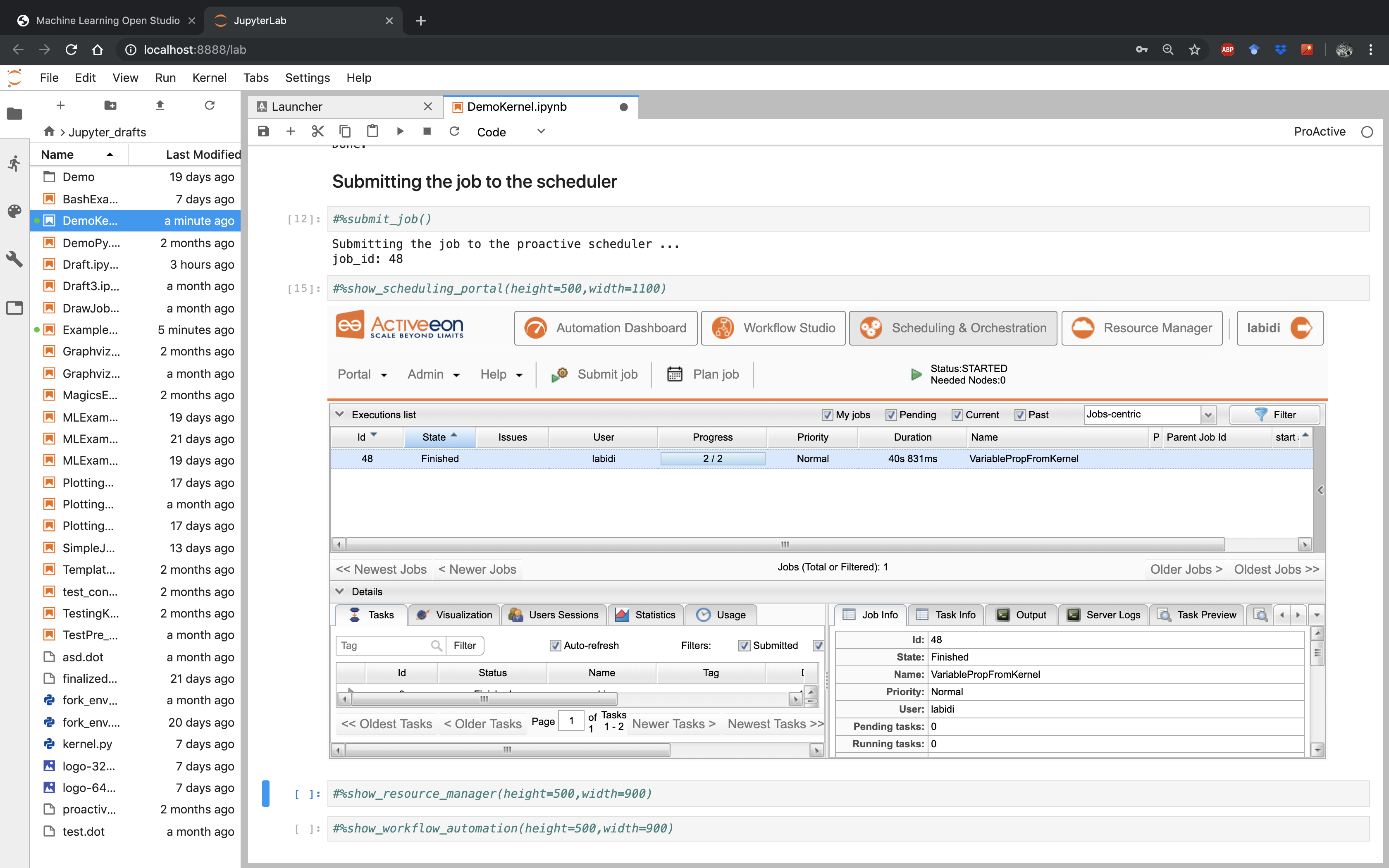
To show the resource manager portal related to the host you are connected to, just run:
#%show_resource_manager([host=YOUR_HOST], [height=HEIGHT_VALUE], [width=WIDTH_VALUE])For the related scheduling portal:
#%show_scheduling_portal([host=YOUR_HOST], [height=HEIGHT_VALUE], [width=WIDTH_VALUE])To monitor your jobs with Workflow Execution inside Jupyter, use:
#%show_workflow_execution([host=YOUR_HOST], [height=HEIGHT_VALUE], [width=WIDTH_VALUE])
The parameters height and width allow the user to adjust the size of the window inside the notebook.
|
10. Customize the ML Bucket
10.1. Create or Update an ML Task
Machine Learning Bucket contains various open source tasks that can be easily used by a simple drag and drop.
It is possible to enrich the ML Bucket by adding your own tasks. (see section 4.3)
It is also possible to customize the code of the generic ML tasks. In this case, you need to drag and drop the targeted task to modify its code in the Task Implementation section.
| It is also possible to add or/and delete variables of each task, set your own fork environments, etc. More details available on ProActive User Guide |
10.2. Set the Fork Environment
A fork execution environment is a new Java Virtual Machine (JVM) which is started exclusively to execute a task. Starting a new JVM means that the task inside it will run in a new environment. This environment can be set up by the creator of the task. A new JVMs is set up with a new classpath, new system properties and more customization.
We used a Docker fork environment for all the ML tasks. activeeon/dlm3 was used as a docker container for all tasks. If your task needs to install new ML libraries which are not available in this container, then, use your own docker container or an appropriate environment with the needed libraries.
| The use of docker containers is recommended as that way other tasks will not be affected by change. Docker containers provide isolation so that the host machine’s software stays the same. More details available on ProActive User Guide |
10.3. Publish a ML Task
The Catalog menu provides the possibility for a user to publish newly created or/and update tasks inside Machine Learning Bucket, you need just to click on Catalog Menu then Publish current Workflow to the Catalog.
Choose machine-leaning Bucket to store your newly added workflow on it.
If the Task with the same name already exists in the 'machine-leaning' bucket, then, it will be updated.
We recommend submitting Tasks with a commit message for easier differentiation between the different submitted versions.
| More details available on ProActive User Guide |
10.4. Create a ML Workflow
The quickstart tutorial on try.activeeon.com shows you how to build a simple workflow using ProActive Studio.
We show below an example of a workflow created with the Studio:
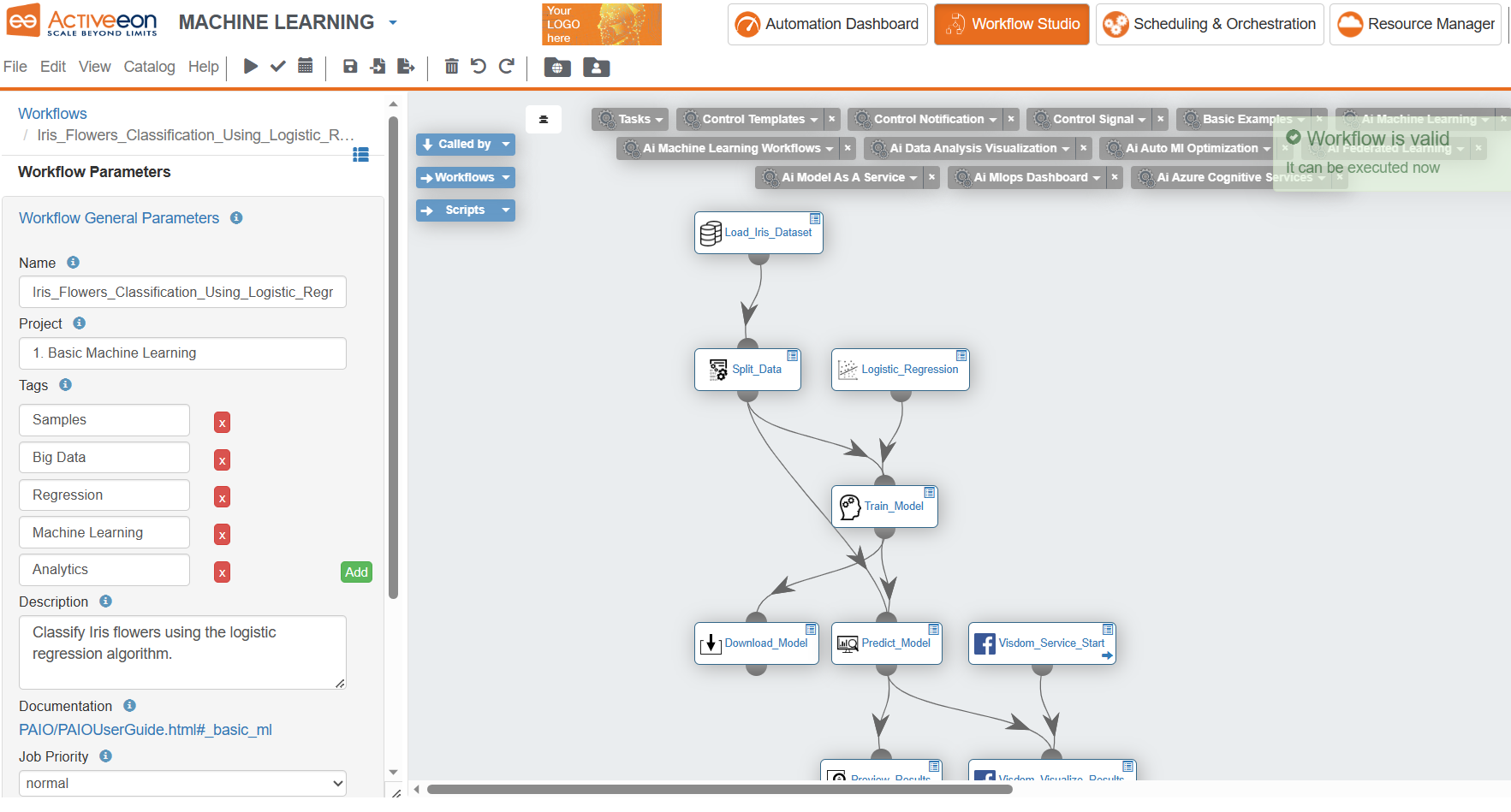
At the left part, are illustrated the General Parameters of the workflow with the following information:
-
Name: the name of the workflow. -
Project: the project name to which belongs the workflow. -
Tags: the tags of the workflow. -
Description: the textual description of the workflow. -
Documentation: if the workflow has a Generic Information named "Documentation", then its URL value is displayed as a link. -
Job Priority: the priority assigned to the workflow. It is by default set toNORMAL, but can be increased or decreased once the job is submitted.
The workflow represented in the above is available on the ai-machine-learning-workflows bucket.
|
11. ML Workflows Examples
The PAIO provides a fast, easy and practical way to execute different workflows using the ML bucket. We present useful ML workflows for different applications in the following subsections.
To test these workflows, you need to add the ai-machine-learning-workflows bucket as main catalog in the ProActive Studio.
-
Open ProActive AI Orchestration home page.
-
Create a new workflow.
-
Change palette preset to
Machine Learning. -
Click on
ai-machine-learningcatalog and pin it open. -
Drag and drop the workflow example of your choice.
-
Execute the chosen workflow, track its progress and preview its results.
More details about these workflows are available in this in ActiveEon’s Auto ML Blog
11.1. Basic ML
The following workflows present some ML basic examples. These workflows are built using generic ML and data visualization tasks available on the ML and Data Visualization buckets.
Diabetics_Detection_using_K_means: trains and tests a clustering model using Mean_shift algorithm.
Vehicle_Type_Using_Model_Explainability: predicts vehicle type based on silhouette measurements, and apply ELI5 and Kernel Explainer to understand the model’s global behavior or specific predictions.
Parallel_Regression_Model_Training: trains three different regression models.
Parallel_Classification_Model_Training: trains three different classification models.
Nested_Cross_Validation: trains a logistic regression model using a nested cross-validation strategies.
Iris_Flowers_Classification_using_Logistic_Regression: trains and tests a predictive model using logistic_regressive algorithm.
House_Price_Prediction_using_Linear_Regression: trains and tests a regression model using Mean_shift algorithm.
11.2. Basic AutoML
The following workflows present some ML basic examples using AutoML generic tasks available in the ai-machine-learning bucket.
Breast_Cancer_Detection_Using_AutoSklearn_Classifier: tests several ML pipelines and selects the best model for Cancer Breast detection.
California_Housing_Prediction_Using_TPOT_Regressor: tests several ML pipelines and selects the best model for California housing prediction.
11.3. Log Analysis
The following workflows are designed to detect anomalies in log files. They are constructed using generic tasks which are available on the ai-machine-learning and ai-data-visualization buckets.
Anomaly_Detection_in_Apache_Logs: detects intrusions in apache logs using a predictive model trained using Support Vector Machines algorithm.
Anomaly_detection_in_HDFS_Blocks: trains and test an anomaly detection model for detecting anomalies in HDFS Blocks.
Anomaly_detection_in_HDFS_Nodes: trains and test an anomaly detection model for detecting anomalies in HDFS Nodes.
Unsupervised_Anomaly_Detection: detects anomalies using an Unsupervised One-Class SVM.
11.4. Data Analytics
The following workflows are designed to feature engineering and fusion.
Data_Fusion_And_Encoding: fuses different data structures.
Data_Anomaly_Detection: detects anomalies on energy consumption by customers.
Diabetics_Results_Visualization_Using_Tableau: visualizes Diabetics Results Using Tableau.
11.5. In Memory Workflows
The following workflows are designed for in-memory execution using IPython. IPython enables all types of parallel applications to be developed, executed, debugged, and monitored interactively. For more details, please visit the ipyparallel website.
In_Memory_Iris_Flowers_Classification: classifies Iris flowers using the logistic regression algorithm. This workflow uses an external IPython Engine for in-memory execution.
Start_IPython_Cluster: starts an IPython parallel computing cluster.
11.6. GPU Accelerated Workflows
The following workflows are designed to train machine learning models on GPU using NVIDIA RAPIDS. This reduces the training time from days to minutes.
Train_Classification_Model_On_GPU: trains a machine learning model for data classification on GPU using NVIDIA RAPIDS.
Train_Multiple_Classification_Models_On_GPU: trains multiple machine learning models for data classification on GPU using NVIDIA RAPIDS.
Train_Multiple_Regression_Models_On_GPU: trains multiple machine learning models for data regression on GPU using NVIDIA RAPIDS.
Train_Regression_Model_On_GPU: trains a machine learning model for data regression on GPU using NVIDIA RAPIDS.
Please find in the table below the list of algorithms which have GPU support and that can be tested using the generic tasks in the ai-machine-learning bucket.
Category |
Algorithm |
|
|
|
|
|
|
|
|
|
|
|
|
|
12. Deep Learning Workflows Examples
PAIO provides a fast, easy and practical way to execute deep learning workflows. In the following subsections, we present useful deep learning workflows for text and image classification and generation.
You can test these workflows by following these steps:
-
Open ProActive AI Orchestration home page.
-
Create a new workflow.
-
Click on
Catalogmenu thenAdd Bucket as Extra Catalog Menuand selectai-deep-learning-workflowsbucket. -
Open this added extra catalog menu and drag and drop the workflow example of your choice.
-
Execute the chosen workflow, track its progress and preview its results.
12.1. Azure Cognitive Services
The following workflows present useful examples composed by pre-built Azure cognitive services available on ai-azure-cognitive-services bucket.
Emotion_Detection_in_Bing_News: is a mashup that searches for images of a person using Azure Bing Image Search then performs an emotion detection using Azure Emotion API.
Sentiment_Analysis_in_Bing_News: is a mashup that searches for news related to a given search term using Azure Bing News API then performs a sentiment analysis using Azure Text Analytics API.
12.2. Microsoft Cognitive Toolkit
The following workflows present useful examples for predictive models training and test using Microsoft Cognitive Toolkit (CNTK).
CNTK_ConvNet: trains a Convolutional Neural Network (CNN) on CIFAR-10 dataset.
CNTK_SimpleNet: trains a 2-layer fully connected deep neural network with 50 hidden dimensions per layer.
GAN_Generate_Fake_MNIST_Images: generates fake MNIST images using a Generative Adversarial Network (GAN).
DCGAN_Generate_Fake_MNIST_Images: generates fake MNIST images using a Deep Convolutional Generative Adversarial Network (DCGAN).
12.3. Mixed Workflows
The following workflow presents an example of a workflow built using pre-built Azure cognitive services tasks available on the ai-azure-cognitive-services bucket and custom AI tasks available on the ai-deep-learning bucket.
Custom_Sentiment_Analysis: is a mashup that searches for news related to a given search term using Azure Bing News API then performs a sentiment analysis using a custom deep learning based pretrained model.
12.4. Training Custom AI Workflows - PyTorch library
This section presents custom AI workflows using tasks available on the ai-deep-learning bucket. Such tasks enable you to train your own AI models by a simple drag and drop of custom AI task.
IMDB_Sentiment_Analysis: trains a model to perform sentiment identification and categorization expressed in a piece of text, especially in order to determine the opinion of IMDB users regarding specific movies [positive or negative]. NOTE: Instead of training a model from scratch, a pre-trained sentiment analysis model is available on this link.
Language_Detection: build an RNN model to perform language detection from a text data.
Train_Image_Classification: trains a model to classify images from ants and bees.
Train_Image_Segmentation: trains a segmentation model using SegNet network on Oxford-IIIT Pet Dataset.
Train_Image_Object_Detection: trains objects using YOLOv3 model on COCO dataset proposed by Microsoft Research.
Deep_Model_Explainability: explains a ResNet-18 model using GradientExplainer.
Search_Train_Image_Classification: queries images from a search engine (Bing or DuckDuckGo) and trains a model to classify them.
12.5. Prediction Custom AI Workflows - PyTorch library
This section presents custom AI workflows using tasks available on the ai-deep-learning bucket. Such tasks enable you to test your own AI models by a simple drag and drop of custom AI task.
Image_Classification: predicts a classification model using ResNet_18 network on Ants_vs_Bees Dataset. The pre-trained image classification model is available on this link.
Fake_Celebrity_Faces_Generation: generates a wild diversity of fake faces using a GAN model that was trained based on thousands of real celebrity photos. The pre-trained GAN model is available on this link.
Image_Segmentation: predicts a segmentation model using SegNet network on Oxford-IIIT Pet Dataset. The pre-trained image segmentation model is available on this link.
Image_Object_Detection: detects objects using a pre-trained YOLOv3 model on COCO dataset proposed by Microsoft Research. The pre-trained model is available on this link.
Search_Classify_Images: queries images into search engine (Bing or DuckDuckGo) and predicts a model to classify rocket_vs_plane images. The pre-trained image classiffication model is available on this link.
12.6. Templates
The following workflows represent python templates that can be used to implement a generic machine learning task.
Horovod_Task: is a template to implement a Horovod task with multi-gpu support.
Horovod_Docker_Task: is a template to implement a Horovod task using a Docker container with multi-gpu support.
Horovod_Slurm_Task: is a template to implement a Horovod task using a native SLURM scheduler with multi-gpu support.
TensorFlow_Task: is a simple TensorFlow task template.
Keras_Task: is a simple Keras task template.
PyTorch_Task: is a simple PyTorch task template.
| It is recommended to use an enabled-GPU node to run the deep learning tasks. |
13. References
13.1. AI Workflows Common Variables
In the following table, you can find the variables that are common between most of the available AI workflows in PAIO associated to their descriptions.
Variable name |
Description |
Type |
|
Name of the Native Scheduler node source to use when the workflow tasks must be deployed inside a cluster such as SLURM, LSF, etc. |
String (default=empty) |
|
Parameters given to the native scheduler (SLURM, LSF, etc) while requesting a ProActive node used to deploy the workflow tasks. |
String (default=empty) |
|
If not empty, the workflow tasks will be run only on nodes belonging to the specified node source. |
String (default=empty) |
|
If not empty, the workflow tasks will be run only on nodes that contains the specified token. |
String (default=empty) |
|
Defines the working directory for the data space used to transfer files automatically between the workflow tasks. |
String |
|
Specifies the container platform to be used for executing the workflow tasks. |
List [no-container, docker, podman, singularity] (default=docker) |
|
If True, it will activate the use of GPU on the selected container platform. |
Boolean (default=True) |
|
Specifies the name of the container image that will be used to run the workflow tasks. |
List [docker://activeeon/dlm3, docker://activeeon/cuda, docker://activeeon/cuda2, docker://activeeon/rapidsai, docker://activeeon/tensorflow:latest, docker://activeeon/tensorflow:latest-gpu] (default=empty) |
13.2. ML Bucket
The ai-machine-learning bucket contains diverse generic ML tasks that enable you to easily compose workflows for predictive models learning and testing. This bucket can be easily customized according to your needs.
This bucket offers different options, you can customize it by adding new tasks or update the existing tasks.
| All ML tasks were implemented using Scikit-learn library. |
13.2.1. Public Datasets
Load_Boston_Dataset
Task Overview: Load and return the Boston House-Prices dataset.
| Features | Targets | Dimensionality | Samples Total |
|---|---|---|---|
Real, positive |
Real 5. -50 |
13 |
506 |
Task Variables:
Variable name |
Description |
Type |
|
If False, the task will be ignored, it will not be executed. |
Boolean (default=True) |
|
Specifies how many rows of the dataframe will be previewed in the browser to check each task results. |
Int (default=-1) ( |
Usage:
-
The Boston House-Prices is a dataset for regression, you can only use it with a regression algorithm, such as Linear Regression and Support Vector Regression.
-
After this task, you can use the Split_Data task to divide the dataset into training and testing sets.
| More information about this dataset can be found here. |
Load_Iris_Dataset
Task Overview: Load and return the iris dataset.
| Features | Classes | Dimensionality | Samples per class | Samples total |
|---|---|---|---|---|
Real, positive |
3 |
4 |
50 |
150 |
Task Variables:
Variable name |
Description |
Type |
|
If False, the task will be ignored, it will not be executed. |
Boolean (default=True) |
|
Specifies how many rows of the dataframe will be previewed in the browser to check each task results. |
Int (default=-1) ( |
Usage:
-
The Iris is a dataset for classification, you can only use it with a classification algorithm, such as Support Vector Machines and Logistic Regression.
-
After this task, you can use the Split_Data task to divide the dataset into training and testing sets.
| More information about this dataset can be found here. |
13.2.2. Input and Output Data
Download_Model
Task Overview: Download a trained model on your computer device.
Task Variables:
Variable name |
Description |
Type |
|
If False, the task will be ignored, it will not be executed. |
Boolean (default=True) |
Usage: It should be used after the task Train_Model.
Export_Data
Task Overview: Export the results of the predictions generated by a classification, clustering or regression algorithm.
Task Variables:
Variable name |
Description |
Type |
|
If False, the task will be ignored, it will not be executed. |
Boolean (default=True) |
|
Converts the prediction results to HTML, HYPER and CSV file. |
String [CSV, JSON, HTML, TABLEAU] |
|
Specifies how many rows of the dataframe will be previewed in the browser to check each task results. |
Int (default=-1) ( |
Usage: It should be used after the task Predict_Model.
Import_Data
Task Overview: Load data from external sources and predict its features types if enabled.
Task Variables:
Variable name |
Description |
Type |
|
If False, the task will be ignored, it will not be executed. |
Boolean (default=True) |
|
Selects the type of data source. |
List [PA:URL,PA:URI,PA:USER_FILE,PA:GLOBAL_FILE] (default=PA:URL) |
|
Inserts a file path/name. |
String |
|
Defines a delimiter to use. |
String (default=;) |
|
Refers to the column "label name". |
String |
|
Specifies how many rows of the dataframe will be previewed in the browser to check each task results. |
Int (-1 means preview all the rows) |
|
If True, the types of the dataset features will be predicted (as numerical or categorical). |
Boolean (default=False) |
| Your CSV file should be in a table format. See the example below. |
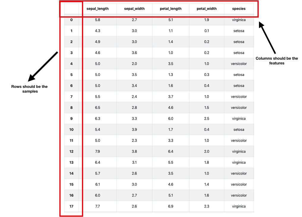
Import_Data_And_Automate_Feature_Engineering
Task Overview: This workflow provides a complete solution to assist data scientists to successfully load and encode their categorical data. It currently supports different encoding methods such as Label, OneHot, Dummy, Binary, Base N, Hash and Target. It also enables:
-
Automatic identification of the best-suited method for encoding each categorical column, when no encoding method is selected (Auto mode).
-
Data type recognition: identification of the data type of each column (categorical or numerical).
-
Creation of summary statistics for each column: missing values, minimum, maximum, average, zeros, and cardinality.
-
Editing of the data structure: modification of column information (name, type, category, etc.), deletion of a column, etc.
This workflow can be used:
-
Stand-alone such that the results can be saved in the User Data Space or locally.
-
In a ML pipeline where the results will be transferred as an input for the following task in the pipeline.
| For further information, please check the subsection AutoFeat. |
Variable name |
Description |
Type |
Task variables |
||
|
Selects the method/protocol to import the data source. |
List [PA:URL,PA:URI,PA:USER_FILE,PA:GLOBAL_FILE] (default=PA:URL) |
|
Inserts the path/name of the file that contains the dataset. |
String |
|
Defines a delimiter to use. |
String (default=;) |
|
Specifies how many rows of the encoded dataframe will be previewed in the workflow results. |
Int (-1 means preview all the rows) |
Import_Model
Task Overview: Load a trained model, and use it to make predictions for new coming data.
Task Variables:
Variable name |
Description |
Type |
|
If False, the task will be ignored, it will not be executed. |
Boolean (default=True) |
|
Type the URL to load your trained model. default: https://s3.eu-west-2.amazonaws.com/activeeon-public/models/pima-indians-diabetes.model |
String |
Usage: It should be used before Predict_Model to make predictions.
Preview_Results
Task Overview: Preview the HTML results of the predictions generated by a classification, clustering or regression algorithm.
Task Variables:
Variable name |
Description |
Type |
|
If False, the task will be ignored, it will not be executed. |
Boolean (default=True) |
|
Specifies how many rows of the dataframe will be previewed in the browser to check each task results. |
Int (default=-1) ( |
|
Converts the prediction results to HTML or CSV file. |
String [CSV, JSON or HTML] |
Usage: It should be used after the task Predict_Model.
Log_Parser
Task Overview: Convert an unstructured raw log file into a structured one by matching a group of event patterns.
Task Variables:
Variable name |
Description |
Type |
|
Put the URL of the raw log file that you need to parse. |
String |
|
Put the URL of the CSV file that contains the different RegEx expressions of each possible pattern and their corresponding variables. The csv file must contain three columns (See the example below): A. id_pattern: Integer Specify the column containing the identifier of each pattern B. Pattern: RegEx expression Define the regex expression of each pattern C. Variables: String Specify the name of each variable included in the pattern. N.B: Use the symbol ‘*’ for variables that you need to neglect. (e.g., in the example below the 5th variable is neglected) N.B: All variables specified in each Regex expressions have to be mentioned in the column « Variables » in the right order (use ',' to separate the variable names). |
String |
|
Indicate the extension of the file where you will save the resulted structured logs. |
String [CSV or HTML] |
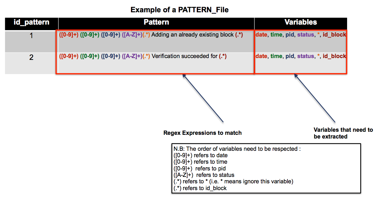
Usage: Could be connected with the tasks Query_Data and Feature_Vector_Extractor.
13.2.3. Data Preprocessing
Append_Data
Task Overview: Append rows of other to the end of this frame, returning a new object. Columns not in this frame are added as new columns.
Task Variables:
Variable name |
Description |
*Type |
|
If False, the task will be ignored, it will not be executed. |
Boolean (default=True) |
Drop_Columns
Task Overview: Drop the columns specified in COLUMNS_NAME variable.
Task Variables:
Variable name |
Description |
Type |
|
If False, the task will be ignored, it will not be executed. |
Boolean (default=True) |
|
The list of columns that need to be dropped. Columns names should be separated by a comma. |
String |
| More details about the source code of this task can be found here. |
Drop_NaNs
Task Overview: Replace inf values to NaNs in a first place then drop objects on a given axis where alternately any or all of the data are missing.
| More details about the source code of this task can be found here. |
Encode_Data
Task Overview: Encode the values of the columns specified in COLUMNS_NAME variable with integer values between 0 and "the number of unique variables"-1.
Task Variables:
Variable name |
Description |
Type |
|
If False, the task will be ignored, it will not be executed. |
Boolean (default=True) |
|
The list of columns that need to be encoded. Columns names should be separated by a comma. |
String |
| More details about the source code of this task can be found here. |
Fill_NaNs
Task Overview: Fill NA/NaN values using the specified method.
Task Variables:
Variable name |
Description |
Type |
|
If False, the task will be ignored, it will not be executed. |
Boolean (default=True) |
|
Refers to the value to use to fill holes (e.g., 0). |
Integer |
| More details about the source code of this task can be found here. |
Filter_Columns
Task Overview: Subset columns of a dataframe according to the specified list of columns in the COLUMNS_NAME variable.
Task Variables:
Variable name |
Description |
Type |
|
If False, the task will be ignored, it will not be executed. |
Boolean (default=True) |
|
The list of columns to restrict to. Columns names should be separated by a comma. |
String |
| More details about the source code of this task can be found here. |
Merge_Data
Task Overview: Merge DataFrame objects by performing a database-style join operation based on a specific reference column specified in the REF_COLUMN variable.
Task Variables:
Variable name |
Description |
Type |
|
If False, the task will be ignored, it will not be executed. |
Boolean (default=True) |
|
The list of columns to restrict to. Columns names should be separated by a comma. |
String |
| More details about the source code of this task can be found here. |
Scale_Data
Task Overview: Scale a dataset based on a robust scaler or standard scaler.
Task Variables:
Variable name |
Description |
Type |
|
If False, the task will be ignored, it will not be executed. |
Boolean (default=True) |
|
The list of columns to restrict to. Columns names should be separated by a comma. |
List [RobustScaler, StandardScaler] (default=RobustScaler) |
|
Specifies how many rows of the dataframe will be previewed in the browser to check each task results. |
Int (default=-1) ( |
|
The list of columns that will be scaled. Column names should be separated by a comma. |
String |
| More details about the source code of this task can be found here. |
Split_Data
Task Overview: Separate data into train and test subsets.
Task Variables:
Variable name |
Description |
Type |
|
If False, the task will be ignored, it will not be executed. |
Boolean (default=True) |
|
This parameter must be float within the range (0.0, 1.0), not including the values 0.0 and 1.0. default = 0.7 |
Float |
| More details about the source code of this task can be found here. |
Rename_Columns
Task Overview: Rename the columns of a data frame.
Task Variables:
Variable name |
Description |
Type |
|
If False, the task will be ignored, it will not be executed. |
Boolean (default=True) |
|
The list of columns that will be renamed. Column names should be separated by a comma. |
String |
Query_Data
Task Overview: Query the columns of your data with a boolean expression.
Task Variables:
Variable name |
Description |
Type |
|
If False, the task will be ignored, it will not be executed. |
Boolean (default=True) |
|
The query string to evaluate. |
String |
|
Refers to the extension of the file where the resulted filtered data will be saved. |
String [CSV or HTML] |
| More details about the source code of this task can be found here. |
13.2.4. Feature Extraction
Summarize_Data
Task Overview: Calculate the histogram of a dataframe based on a reference column that need to be specified in the variable REF_COLUMN.
Task Variables:
Variable name |
Description |
Type |
|
If False, the task will be ignored, it will not be executed. |
Boolean (default=True) |
|
The model that will be used to summarize data. |
List [KMeans, PolynomialFeatures] (default=KMeans) |
|
The column that will be used to group by the different histogram measures. |
String |
| More details about the source code of this task can be found here. |
Tsfresh_Features_Extraction
Task Overview: Calculate a comprehensive number of time series features based on the library TSFRESH.
Task Variables:
Variable name |
Description |
Type |
|
If False, the task will be ignored, it will not be executed. |
Boolean (default=True) |
|
The column that contains the values of the time series |
String |
|
The column that will be used to group by the different features. |
String |
|
False if you do not need to extract all the possible features extractable by the library TSFRESH. |
Boolean (default = False) |
|
Specifies how many rows of the dataframe will be previewed in the browser to check each task results. |
Int (default=-1) ( |
| More details about the source code of this task can be found here. |
Feature_Vector_Extractor
Task Overview: Encode structured data into numerical feature vectors whereby ML models can be applied.
Task Variables:
Variable name |
Description |
Type |
|
If False, the task will be ignored, it will not be executed. |
Boolean (default=True) |
|
The ID of the entity that you need to represent (to group by). |
String |
|
The extension of the file where the resulted features will be saved. |
String [CSV or HTML] |
|
The index of column containing the log patterns.[specific to features extraction from logs]. |
String |
|
True if you need to extract count the number of occurrence of each pattern per session. |
Boolean [True or False] |
|
The different variables that need to be considered to extract features according to their content. N.B: separate the different variables with a comma ',' |
String |
|
Refers to the different variables that need to be considered to count their distinct content. |
String N.B: separate the different variables with a comma ',' |
|
True if you need to extract state and count features per session. |
Boolean [True or False] |
Usage: Could be connected with Train_Model if you need to train a model using unsupervised ML techniques.
13.2.5. AutoML
TPOT_Classifier
Task Overview: TPOT_Classifier performs an intelligent search over ML pipelines that can contain supervised classification models, preprocessors, feature selection techniques, and any other estimator or transformer that follows the scikit-learn API.
Task Variables:
Variable name |
Description |
Type |
|
If True, This task code will be executed. |
Boolean (default=True) |
|
Number of iterations to the run pipeline optimization process. |
Integer (default=3) |
|
Function used to evaluate the quality of a given pipeline for the classification problem. |
List (default=accuracy) |
|
Cross-validation strategy used when evaluating pipelines. |
Integer (default=5) |
|
How much information TPOT communicates while it’s running. Possible inputs: 0, 1, 2, 3. |
Integer (default=1) |
Usage: It should be connected with Train_Model.
| More information about this task can be found here. |
AutoSklearn_Classifier
Task Overview: AutoSklearn_Classifier leverages recent advantages in Bayesian optimization, meta-learning and ensemble construction to performs an intelligent search over ML classification algorithms.
Task Variables:
Variable name |
Description |
Type |
|
If True, This task code will be executed. |
Boolean (default=True) |
|
Time limit in seconds for the search of appropriate models. |
Integer (default=30) |
|
Time limit for a single call to the ML model. Model fitting will be stopped if the ML algorithm runs over the time limit. |
Integer (default=27) |
|
If True, the defined resampling strategy will be applied. |
Boolean (default=True) |
|
Strategy to handle overfitting. |
String (default='cv') |
|
Number of folds for cross-validation. |
Integer (default=5) |
Usage: It should be connected with Train_Model.
|
TPOT_Regressor
Task Overview: TPOT_Regressor performs an intelligent search over ML pipelines that can contain supervised regression models, preprocessors, feature selection techniques, and any other estimator or transformer.
Task Variables:
Variable name |
Description |
Type |
|
If True, This task code will be executed. |
Boolean (default=True) |
|
Number of iterations to the run pipeline optimization process. |
Integer (default=3) |
|
Function used to evaluate the quality of a given pipeline for the regression problem. |
List (default=neg_mean_squared_error) |
|
Cross-validation strategy used when evaluating pipelines. |
Integer (default=5) |
|
How much information TPOT communicates while it’s running. Possible inputs: 0, 1, 2, 3. |
Integer (default=1) |
Usage: It should be connected with Train_Model .
| More information about this task can be found here. |
AutoSklearn_Regressor
Task Overview: AutoSklearn_Regressor leverages recent advantages in Bayesian optimization, meta-learning and ensemble construction to performs an intelligent search over ML regression algorithms.
Task Variables:
Variable name |
Description |
Type |
|
If True, This task code will be executed. |
Boolean (default=True) |
|
Time limit in seconds for the search of appropriate models. |
Integer (default=120) |
|
Time limit for a single call to the ML model. Model fitting will be stopped if the ML algorithm runs over the time limit. |
Integer (default=30) |
|
If True, the defined resampling strategy will be applied. |
Boolean (default=False) |
|
Strategy to handle overfitting. |
String (default='cv') |
|
Number of folds for cross-validation. |
Integer (default=5) |
Usage: It should be connected with Train_Model .
| More information about this task can be found here. |
13.2.6. ML Classification
Gaussian_Naive_Bayes
Task Overview: Naive Bayes classifier is a family of simple probabilistic classifier based on applying Bayes' theorem with strong (naive) independence assumptions between the features.
Task Variables:
Variable name |
Description |
Type |
|
If False, the task will be ignored, it will not be executed. |
Boolean (default=True) |
|
Specifies the parameters' values of the gaussian naive bayes algorithm. Check the list of parameters here. |
JSON format |
Usage: It should be connected with Train_Model or Predict_Model.
| More information about this task can be found here. |
Logistic_Regression
Task Overview: Logistic Regression is a regression model where the Dependent Variable (DV) is categorical.
Task Variables:
Variable name |
Description |
Type |
|
If False, the task will be ignored, it will not be executed. |
Boolean (default=True) |
|
Specifies the parameters' values of the logistic regression algorithm. Check the list of parameters here. |
JSON format |
Usage: It should be connected with Train_Model and Predict_Model.
| More information about the source code of this task can be found here. |
Support_Vector_Machines
Task Overview: Support vector machines are supervised learning models with associated learning algorithms that analyze data used for classification.
Task Variables:
Variable name |
Description |
Type |
|
If False, the task will be ignored, it will not be executed. |
Boolean (default=True) |
|
Specifies the parameters' values of the support vector machines algorithm. Check the list of parameters here. |
JSON format |
Usage: It should be connected with Train_Model and Predict_Model.
| More information about the source of this task can be found here. |
13.2.7. ML Regression
Bayesian_Ridge_Regression
Task Overview: Bayesian linear regression is an approach to linear regression in which the statistical analysis is undertaken within the context of Bayesian inference.
Task Variables:
Variable name |
Description |
Type |
|
If False, the task will be ignored, it will not be executed. |
Boolean (default=True) |
|
Specifies the parameters' values of the bayesian ridge regression algorithm. Check the list of parameters here. |
JSON format |
Usage: It should be connected with Train_Model and Predict_Model.
| More information about the source of this task can be found here. |
Linear_Regression
Task Overview: Linear regression is a linear approach for modeling the relationship between a scalar dependent variable y and one or more explanatory variables (or independent variables) denoted X.
Task Variables:
Variable name |
Description |
Type |
|
If False, the task will be ignored, it will not be executed. |
Boolean (default=True) |
|
Specifies the parameters' values of the linear regression algorithm. Check the list of parameters here. |
JSON format |
Usage: IT should be connected with Train_Model and Predict_Model.
| More information about the source of this task can be found here. |
Support_Vector_Regression
Task Overview: Support vector regression are supervised learning models with associated learning algorithms that analyze data used for regression.
Task Variables:
Variable name |
Description |
Type |
|
If False, the task will be ignored, it will not be executed. |
Boolean (default=True) |
|
Specifies the parameters' values of the support vector regression algorithm. Check the list of parameters here. |
JSON format |
Usage: It should be connected with Train_Model and Predict_Model.
| More information about the source of this task can be found here. |
13.2.8. ML Anomaly Detection
Isolation_Forest
Task Overview: Isolation Forest is an outlier detection method which returns the anomaly score of each sample using the IsolationForest algorithm. The IsolationForest ‘isolates’ observations by randomly selecting a feature and then randomly selecting a split value between the maximum and minimum values of the selected feature.
Task Variables:
Variable name |
Description |
Type |
|
If False, the task will be ignored, it will not be executed. |
Boolean (default=True) |
|
Specifies the parameters' values of the isolation forest algorithm. Check the list of parameters here. |
JSON format |
| More information about the source of this task can be found here. |
One_Class_SVM
Task Overview: One-class SVM is an algorithm that learns a decision function for novelty detection: classifying new data as similar or different to the training set.
Task Variables:
Variable name |
Description |
Type |
|
If False, the task will be ignored, it will not be executed. |
Boolean (default=True) |
|
Specifies the parameters' values of the one class algorithm. Check the list of parameters here. |
JSON format |
| More information about the source of this task can be found here. |
13.2.9. ML Clustering
K_Means
Task Overview: K-means clustering aims to partition n observations into k clusters in which each observation belongs to the cluster with the nearest mean, serving as a prototype of the cluster
Task Variables:
Variable name |
Description |
Type |
|
If False, the task will be ignored, it will not be executed. |
Boolean (default=True) |
|
Specifies the parameters' values of the K-means algorithm. Check the list of parameters here. |
JSON format |
Usage: It should be connected with Train_Model and Predict_Model.
| More information about the source of this task can be found here. |
Mean_Shift
Task Overview: Mean shift is a non-parametric feature-space analysis technique for locating the maxima of a density function.
Task Variables:
Variable name |
Description |
Type |
|
If False, the task will be ignored, it will not be executed. |
Boolean (default=True) |
|
Specifies the parameters' values of the Mean Shift algorithm. Check the list of parameters here. |
JSON format |
Usage: It should be connected with Train_Model and Predict_Model.
| More information about the source of this task can be found here. |
13.2.10. ML Ensemble Learning
AdaBoost
Task Overview: AdaBoost combines weak classifier algorithm into a single strong classifier.
Task Variables:
Variable name |
Description |
Type |
|
If False, the task will be ignored, it will not be executed. |
Boolean (default=True) |
|
Specifies the parameters' values of the AdaBoost algorithm. Check the list of parameters here. |
JSON format |
|
Specifies the type of algorithm. |
List [Classification or Regression] |
Usage: It should be connected with Train_Model and Predict_Model.
| More information about the source of this task can be found here. |
CatBoost
Task Overview: CatBoost is a gradient boosting which helps to reduce overfitting. It can be used to solve both classification and regression challenge.
Task Variables:
Variable name |
Description |
Type |
|
If False, the task will be ignored, it will not be executed. |
Boolean (default=True) |
|
Specifies the parameters' values of the CatBoost algorithm. Check the list of parameters here. |
JSON format |
|
Specifies the type of algorithm. |
List [Classification or Regression] |
Usage: It should be connected with Train_Model and Predict_Model.
| More information about the source of this task can be found here. |
Gradient_Boosting
Task Overview: Gradient Boosting is an algorithm for regression and classification problems. It produces a prediction model in the form of an ensemble of weak prediction models. Task Variables:
Variable name |
Description |
Type |
|
If False, the task will be ignored, it will not be executed. |
Boolean (default=True) |
|
Specifies the parameters' values of the Gradient Boosting algorithm. Check the list of parameters here. |
JSON format |
|
Specifies the type of algorithm. |
List [Classification or Regression] |
Usage: It should be connected with Train_Model and Predict_Model.
| More information about the source of this task can be found here. |
Random_Forest
Task Overview: Random Forest is an algorithm for regression, classification and other tasks that operates by constructing a multitude of decision trees at training time. Task Variables:
Variable name |
Description |
Type |
|
If False, the task will be ignored, it will not be executed. |
Boolean (default=True) |
|
Specifies the parameters' values of the Random Forest algorithm. Check the list of parameters here. |
JSON format |
|
Specifies the type of algorithm. |
List [Classification or Regression] |
Usage: It should be connected with Train_Model and Predict_Model.
| More information about the source of this task can be found here. |
XGBoost
Task Overview: XGBoost is an implementation of gradient boosted decision trees designed for speed and performance.
Task Variables:
Variable name |
Description |
Type |
|
If False, the task will be ignored, it will not be executed. |
Boolean (default=True) |
|
Specifies the parameters' values of the XGBoost algorithm. Check the list of parameters here. |
JSON format |
|
Specifies the type of algorithm. |
List [Classification or Regression] |
Usage: It should be connected with Train_Model and Predict_Model.
| More information about the source of this task can be found here. |
13.2.11. Train
Train_Model
Task Overview: Train a model using a classification, a regression or an anomaly algorithm.
Variable name |
Description |
Type |
|
If False, the task will be ignored, it will not be executed. |
Boolean (default=True) |
|
Refers to the column "label name". |
String |
|
Enables NVIDIA RAPIDS support. |
Boolean (default=False) |
Usage: It should be used after a classification, a regression or an anomaly algorithm, such as Support_Vector_Machines, Gaussian_Naive_Bayes, Linear_Regression, Bayesian_Ridge_Regression, Linear_Regression, Support_Vector_Regression, Isolation_Forest, One_Class_SVM, AdaBoost, CatBoost, Gradient_Boosting, Random_Forest, and XGBoost.
13.2.12. Predict
Predict_Model
Task Overview: Generate predictions using a trained model.
Variable name |
Description |
Type |
|
If False, the task will be ignored, it will not be executed. |
Boolean (default=True) |
|
Refers to the column "label name". |
String. |
|
Enables NVIDIA RAPIDS support. |
Boolean (default=False) |
Usage: It should be used after the task Train_Model.
13.2.13. ML Explainability
Model_Explainability
Task Overview: Explain ML models globally on all data, or locally on a specific data point using the SHAP and eli5 Python libraries.
Variable name |
Description |
Type |
|
If False, the task will be ignored, it will not be executed. |
Boolean (default=True) |
|
Refers to the column "label name". |
String |
|
Partial Dependence Plots show how a feature affects predictions. |
String [e.g., distance_circularity, max_length_aspect_ratio, etc]. |
|
2D Partial Dependence Plots show predictions for any combination of two features. |
String [e.g, distance_circularity, max_length_aspect_ratio]. |
|
Defines the row of data to show. |
Integer |
Usage: It should be connected with Train_Model.
| The SHAP values interpret the impact of having a certain value for a given feature in comparison to the prediction we would make if that feature took some baseline value. Feature values causing increased predictions are in pink and Feature values decreasing the prediction are in blue. |
| More information about the source of the SHAP and eli5 Python libraries can be found here. |
13.3. Deep Learning Bucket
The ai-deep-learning bucket contains diverse generic deep learning tasks that enable you to easily compose workflows for predictive models learning and testing. This bucket can be easily customized according to your needs.
It offers different options, you can customize it by adding new tasks or update the existing tasks.
|
13.3.1. Input and Output
Import_Image_Dataset
Task Overview: Load and return an image dataset. There are some simple rules for organizing your files and folders.
-
Image Classification Dataset: Each class must have its own folder which should contain its related images. The Figure below shows how your folders and files should be organized.
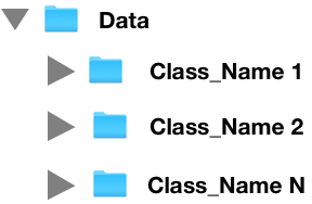
| You can use RGB images in JPG or PNG formats. |
| You can find an example of the organization of the folders at: https://s3.eu-west-2.amazonaws.com/activeeon-public/datasets/ants_vs_bees.zip |
-
Image Segmentation Dataset: Two folders are required: the first folder should contain the RGB images in JPG format and another folder should contain its corresponding annotations in PASCAL VOC format. RGB images and annotations should be organized as follows:

| You can use RGB images in JPG format (Images folder) and the groundtruth annotations (Classes folder) in the PNG format using Pascal VOC pattern. |
| You can find an example of the organization of the folders at: https://s3.eu-west-2.amazonaws.com/activeeon-public/datasets/oxford.zip |
-
Object Detection Dataset: Two folders are demanded: the first folder should contain the RGB images in JPG format and another folder should contain its corresponding anotations in XML format using PASCAL VOC format or TXT format using YOLO format. The RGB images and annotations should be organized as follows:

| You can use RGB images in JPG format (Images folder) and the annotations (Classes folder) in the XML format using Pascal VOC or COCO pattern. |
| In these links, you can find an example of the organization of the folders using Pascal_VOC Dataset and COCO Dataset. |
Task Variables:
Variable name |
Description |
Type |
|
If True, the tasks will be executed on GPU nodes. |
Boolean (default=True) |
|
Selects the type of data source. |
List [PA:URL,PA:URI,PA:USER_FILE,PA:GLOBAL_FILE] (default=PA:URL) |
|
Inserts a file path/name. |
String |
|
Must be a float within the range (0.0, 1.0), not including the values 0.0 and 1.0. |
Float (default=1) |
|
Must be a float within the range (0.0, 1.0), not including the values 0.0 and 1.0. |
Float (default=0.1) |
|
Must be a float within the range (0.0, 1.0), not including the values 0.0 and 1.0. |
Float (default=0.3) |
|
Enter the type of your dataset. There are two possible types: classification or segmentation |
List [Classification, Detection or Segmentation] |
Usage: It should be connected with Train_Image_Segmentation_Model, Train_Image_Classification_Model or Predict_Image_Classification_Model, Predict_Image_Segmentation_Model.
Download_Model
Task Overview: Download a trained model by a deep learning algorithm.
Task Variables:
Variable name |
Description |
Type |
|
If True, the tasks will be executed on GPU nodes. |
Boolean (default=True) |
|
Choose the type of your model. There are two possible types: PyTorch or ONNX. |
List [PyTorch or ONNX] |
| Not all deep networks support the ONNX model yet. You can download ONNX model of the following networks: AlexNet, DenseNet-161, ResNet-18, VGG-16 and YOLO. |
Usage: It should be connected with Train_Image_Classification_Model or Train_Text_Classification_Model or Train_Image_Segmentation_Model or Train_Image_Object_Detection_Model.
Import_Model
Task Overview: Import a trained model by a deep learning algorithm.
Task Variables:
Variable name |
Description |
Type |
|
If True, the tasks will be executed on GPU nodes. |
Boolean (default=True) |
|
URL pointing to the zip folder containing the needed model. |
String |
Usage: It should be connected with Predict_Text_Classification_Model or Predict_Image_Classification_Model or Predict_Image_Segmentation_Model.
Import_Text_Dataset
Task Overview: Import data from external sources. Each unique label must have its own folder which should contain its related text file. If your data is unlabeled, use the name 'unlabeled' for the folder containing your text file.
Task Variables:
Variable name |
Description |
Type |
|
If True, the tasks will be executed on GPU nodes. |
Boolean (default=True) |
|
URL pointing to the zip folder containing the needed data. |
String |
|
Must be a float within the range (0.0, 1.0), not including the values 0.0 and 1.0. |
Float (default=1) |
|
Must be a float within the range (0.0, 1.0), not including the values 0.0 and 1.0. |
Float (default=0.3) |
|
Must be a float within the range (0.0, 1.0), not including the values 0.0 and 1.0. |
Float (default=0.1) |
|
Use a subset of the data to train the model fastly. |
Boolean (default=True) |
|
Transform the text into tokens. Different options are available (str.split, moses, spacy, revtok, subword) |
List (default=str.split) |
|
Split the text into separated paragraphs, separated lines, separated words. Choose your own separator. |
String (default=\r) |
|
Encode to be used to read the text. |
String (default='utf-8') |
|
True if data is labeled. |
Boolean (default=True) |
Usage: It should be connected with Train_Text_Classification_Model or Predict_Text_Classification_Model.
| Torchtext were used to preprocess and load the text input. More information about this library can be found here. |
Preview_Results
Task Overview: Preview the results of the predictions generated by the trained model.
Task Variables:
Variable name |
Description |
Type |
|
If True, the tasks will be executed on GPU nodes. |
Boolean (default=True) |
|
Converts the prediction results to HTML or CSV file. |
List (default='HTML') |
Usage: It should be used after the tasks Predict_Text_Classification_Model or Predict_Image_Classification_Model or Predict_Image_Segmentation_Model.
Export_Images
Task Overview: Download a zip file of your results.
Variable name |
Description |
Type |
|
If True, the tasks will be executed on GPU nodes. |
Boolean (default=True) |
Usage: It should be connected to Predict_Image_Classification_Model or Predict_Image_Segmentation_Model.
Search_Image_Dataset
Task Overview: Search image from Bing or DuckDuckGo navigator and return an image dataset.
Task Variables:
Variable name |
Description |
Type |
|
If True, the tasks will be executed on GPU nodes. |
Boolean (default=True) |
|
Specifies the path where the data should be downloaded. |
String |
|
Enters a keyword to query into search engine. |
String |
|
Maximum number of search results for a single query (maximum of 34 per request for Bing navigator). |
List [Bing, DuckDuckGo] default=DuckDuckGo |
|
Inserts (width, height) of the images as a tuple with 2 elements. |
Integer (default=(200, 200)) |
|
Defines a source engine to query and download images. |
String |
Usage: It should be connected with Import_Image_Dataset.
| Torchtext were used to preprocess and load the text input. More information about this library can be found here. |
13.3.2. Image Classification
AlexNet
Task Overview: AlexNet is the name of a Convolutional Neural Network (CNN), originally written with CUDA to run with GPU support, which competed in the ImageNet Large Scale Visual Recognition Challenge in 2012.
Usage: It should be connected to Train_Image_Classification_Model.
Variable name |
Description |
Type |
|
If True, the tasks will be executed on GPU nodes. |
Boolean (default=True) |
|
Parameter to use a pre-trained model for training. If True, the pre-trained model with the corresponding number of layers is loaded and used for training. Otherwise, the network is trained from scratch. |
Boolean (default=True) |
| PyTorch is used to build the model architecture based on AlexNet. |
DenseNet-161
Task Overview: Densely Connected Convolutional Network (DenseNet) is a network architecture where each layer is directly connected to every other layer in a feed-forward fashion (within each dense block).
Usage: It should be connected to Train_Image_Classification_Model.
| PyTorch is used to build the model architecture based on DenseNet-161. |
Variable name |
Description |
Type |
|
If True, the tasks will be executed on GPU nodes. |
Boolean (default=True) |
|
Parameter to use a pre-trained model for training. If True, the pre-trained model with the corresponding number of layers is loaded and used for training. Otherwise, the network is trained from scratch. |
Boolean (default=True) |
ResNet-18
Task Overview: Deep Residual Networks (ResNet-18) is a deep convolutional neural network, trained on 1.28 million ImageNet training images, coming from 1000 classes.
Usage: It should be connected to Train_Image_Classification_Model.
| PyTorch is used to build the model architecture based on ResNet-18. |
Variable name |
Description |
Type |
|
If True, the tasks will be executed on GPU nodes. |
Boolean (default=True) |
|
Parameter to use a pre-trained model for training. If True, the pre-trained model with the corresponding number of layers is loaded and used for training. Otherwise, the network is trained from scratch. |
Boolean (default=True) |
VGG-16
Task Overview: The VGG-16 is an image classification convolutional neural network.
Usage: It should be connected to Train_Image_Classification_Model.
| PyTorch is used to build the model architecture based on VGG-16. |
Variable name |
Description |
Type |
|
If True, the tasks will be executed on GPU nodes. |
Boolean (default=True) |
|
Parameter to use a pre-trained model for training. If True, the pre-trained model with the corresponding number of layers is loaded and used for training. Otherwise, the network is trained from scratch. |
Boolean (default=True) |
13.3.3. Image Segmentation
FCN
Task Overview: The FCN16 combines layers of the feature hierarchy and refines the spatial precision of the output.
Usage: It should be connected to Train_Image_Segmentation_Model.
| PyTorch is used to build the model architecture based on FCN. |
Variable name |
Description |
Type |
|
If True, the tasks will be executed on GPU nodes. |
Boolean (default=True) |
|
Insert (width, height) of the images as a tuple with 2 elements. |
Integer (default=(64, 64)) |
|
Number of classes. |
Integer (default=5) |
SegNet
Task Overview: is a deep convolutional encoder-decoder architecture for robust semantic pixel-wise labelling.
Usage: It should be connected to Train_Image_Segmentation_Model.
| PyTorch is used to build the model architecture based on SegNet. |
Variable name |
Description |
Type |
|
If True, the tasks will be executed on GPU nodes. |
Boolean (default=True) |
|
Insert (width, height) of the images as a tuple with 2 elements. |
Integer (default=(64, 64)) |
|
Number of classes. |
Integer (default=3) |
UNet
Task Overview: consists of a contracting path to capture context and a symmetric expanding path that enables precise localization.
Usage: It should be connected to Train_Image_Segmentation_Model.
| PyTorch is used to build the model architecture based on UNet. |
Variable name |
Description |
Type |
|
If True, the tasks will be executed on GPU nodes. |
Boolean (default=True) |
|
Insert (width, height) of the images as a tuple with 2 elements. |
Integer (default=(64, 64)) |
|
Number of classes. |
Integer (default=3) |
13.3.4. Image Object Detection
SSD
Task Overview: produces a fixed-size collection of bounding boxes and scores for the presence of object class instances in those boxes, followed by a non-maximum suppression step to produce the final detections. For more details click on this link
Usage: It should be connected to Train_Image_Object_Detection_Model.
| PyTorch is used to build the model architecture based on SSD. |
Variable name |
Description |
Type |
|
If True, the tasks will be executed on GPU nodes. |
Boolean (default=True) |
|
Initial iteration. |
Integer (default=0) |
|
Maximum iteration. |
Integer (default=5) |
|
Learning steps update for SGD (Stochastic Gradient Descent). |
Integer (default=5) |
|
Learning rate update for SGD. |
Float (default= 1e-3) Range in [0, 1]. |
|
Gamma update for SGD. |
Float (default=0.1) Range in [0, 1]. |
|
Minimum object size for detection by specifying numerical values or reference areas on screen. Objects smaller than that are ignored. |
Integer (default= [30, 60, 111, 162, 213, 264]) |
|
Maximum object size for detection by specifying numerical values or reference areas on screen. Objects larger than that are ignored. |
Integer (default= [60, 111, 162, 213, 264, 315]) |
|
Initial learning rate. |
Float (default= 1e-8) Range in [0, 1]. |
|
Momentum value for optimization. |
Float (default=0.9) Range in [0, 1]. |
|
Weight decay for SGD |
Float (default= 5e-4) Range in [0, 1]. |
|
Insert (width, height) of the images as a tuple with 2 elements. |
Integer (default=(300, 300)) |
|
Number of classes. |
Integer (default=21) |
|
The URL of the file containing the class names of the dataset. |
String (default=(https://s3.eu-west-2.amazonaws.com/activeeon-public/datasets/voc.names)) |
|
Parameter to use pre-trained model for training. If True, the pre-trained model with the corresponding number of layers is loaded and used for training. Otherwise, the network is trained from scratch. |
Boolean (default=True) |
| The default parameters of the SSD network were set for the PASCAL VOC dataset (http://host.robots.ox.ac.uk/pascal/VOC/voc2012/). If you’d like to use another dataset, you probably need to change the default parameters. |
YOLO
Task Overview: You only look once (YOLO) is a single neural network to predict bounding boxes and class probabilities. For more details click on this link
Usage: It should be connected to Train_Image_Object_Detection_Model.
| PyTorch is used to build the model architecture based on YOLO. |
Variable name |
Description |
Type |
|
If True, the tasks will be executed on GPU nodes. |
Boolean (default=True) |
|
Initial learning rate |
Float (default= 0.0005) Range in [0, 1]. |
|
Momentum value for optimization. |
Float (default=0.9) Range in [0, 1]. |
|
Weight decay for SGD |
Float (default= 5e-4) Range in [0, 1]. |
|
Insert (width, height) of the images as a tuple with 2 elements. |
Integer (default=(414, 416)) |
|
Number of classes. |
Integer (default=81) |
|
This parameter shows how certain it is that the predicted bounding box actually encloses some object. This score does not say anything about what kind of object is in the box, just if the shape of the box is any good. |
Float (default=0.5) Range in [0, 1]. |
|
This parameter will select only the most accurate (highest probability) one of the boxes. |
Float (default=0.45) Range in [0, 1]. |
|
The URL of the file containing the class names of the dataset. |
String (default=(https://s3.eu-west-2.amazonaws.com/activeeon-public/datasets/coco.names)) |
|
Parameter to use pre-trained model for training. If True, the pre-trained model with the corresponding number of layers is loaded and used for training. Otherwise, the network is trained from scratch. |
Boolean (default=True) |
| The default parameters of the YOLO network were set for the COCO dataset (https://cocodataset.org/#home). If you’d like to use another dataset, you probably need to change the default parameters. |
13.3.5. Text Classification
GRU
Task Overview: Gated recurrent units (GRUs) are a gating mechanism in recurrent neural networks.
Task Variables:
Variable name |
Description |
Type |
|
If True, the tasks will be executed on GPU nodes. |
Boolean (default=True) |
|
The dimension of the vectors that will be used to map words in some languages. |
Integer (default=50) |
|
Hidden dimension of the neural network. |
Integer (default=40) |
|
Percentage of the neurons that will be ignored during the training. |
Float (default=0.5) |
Usage: It should be connected to Train_Text_Classification_Model.
| PyTorch is used to build the model architecture based on GRU. |
LSTM
Task Overview: Long short-term memory (LSTM) units (or blocks) are a building unit for layers of a recurrent neural network (RNN).
Task Variables:
Variable name |
Description |
Type |
|
If True, the tasks will be executed on GPU nodes. |
Boolean (default=True) |
|
The dimension of the vectors that will be used to map words in some languages. |
Integer (default=50) |
|
Hidden dimension of the neural network. |
Integer (default=40) |
|
Percentage of the neurons that will be ignored during the training. |
Float (default=0.5) |
HUsage: It should be connected to Train_Text_Classification_Model.
| PyTorch is used to build the model architecture based on LSTM. |
RNN
Task Overview: A recurrent neural network (RNN) is a class of artificial neural network where connections between units form a directed graph along a sequence.
Task Variables:
Variable name |
Description |
Type |
|
If True, the tasks will be executed on GPU nodes. |
Boolean (default=True) |
|
The dimension of the vectors that will be used to map words in some languages. |
Integer (default=50) |
|
Hidden dimension of the neural network. |
Integer (default=40) |
|
Percentage of the neurons that will be ignored during the training. |
Float (default=0.5) |
Usage: It should be connected to Train_Text_Classification_Model.
| PyTorch is used to build the model architecture based on RNN. |
13.3.6. Train Model
Train_Image_Classification_Model
Task Overview: Train a model using a Convolutional Neural Network (CNN) algorithm.
Task Variables:
Variable name |
Description |
Type |
|
If True, the tasks will be executed on GPU nodes. |
Boolean (default=True) |
|
Number of times all the training vectors are used once to update the weights. |
Integer (default=1) |
|
Batch size to be used. |
Integer (default=4) |
|
Number of subprocesses to use for data loading. 0 means that the data will be loaded in the main process. |
Integer (default=2) |
|
Set to True to have the data reshuffled at every epoch. |
Boolean (default=True)se for data loading. 0 means that the data will be loaded in the main process. |
Usage: Could be connected to Predict_Image_Classification_Model and Download_Model.
Train_Text_Classification_Model
Task Overview: Train a model using a Recurrent Neural Network (RNN) algorithm.
Task Variables:
Variable name |
Description |
Type |
|
If True, the tasks will be executed on GPU nodes. |
Boolean (default=True) |
|
Determines how quickly or how slowly you want to update the parameters. |
Float (default=0.001) |
|
Choose the optimization algorithm that would help you to minimize the Loss function. Different options are available (42B, 840B, twitter.27B,6B). |
List (default=Adam) |
|
Choose the function that will be used to compute the loss. Different options are available (Adam,RMS, SGD, Adagrad, Adadelta). |
List (default=NLLLoss) |
|
Number of times all the training vectors are used once to update the weights. |
Integer (default=10) |
|
True if you want to update the embedding vectors during the training process. |
Boolean (default=False) |
|
Choose the glove vectors that need to be used for words embedding. Different options are available (42B, 840B, twitter.27B,6B) |
List (default=6B) |
|
True if you need to execute the training task in a GPU node. |
Boolean (default=True) |
Usage: Could be connected to Predict_Text_Classification_Model and Download_Model.
Train_Image_Segmentation_Model
Task Overview: Train a model using an image segmentation algorithm.
Task Variables:
Variable name |
Description |
Type |
|
If True, the tasks will be executed on GPU nodes. |
Boolean (default=True) |
|
Number of times all the training vectors are used once to update the weights. |
Integer (default=1) |
|
Batch size to be used. |
Integer (default=1) |
|
Number of subprocesses to use for data loading. |
Integer (default=1) |
|
Set to True to have the data reshuffled at every epoch. |
Boolean (default=True)se for data loading. 0 means that the data will be loaded in the main process. |
Usage: Could be connected to Predict_Image_Segmentation_Model and Download_Model.
Train_Image_Object_Detection_Model
Task Overview: Train a model using an object detection algorithm.
Task Variables:
Variable name |
Description |
Type |
|
If True, the tasks will be executed on GPU nodes. |
Boolean (default=True) |
|
Number of times all the training vectors are used once to update the weights. |
Integer (default=1) |
|
Batch size to be used. |
Integer (default=1) |
|
Number of subprocesses to use for data loading. |
Integer (default=1) |
13.3.7. Predict
Predict_Image_Classification_Model
Task Overview: Generate predictions using a trained model.
Variable name |
Description |
Type |
|
If True, the tasks will be executed on GPU nodes. |
Boolean (default=True) |
|
Batch size to be used. |
Integer (default=4) |
|
Number of subprocesses to use for data loading. |
Integer (default=2) |
|
Set to True to have the data reshuffled at every epoch. |
Boolean (default=True) for data loading. |
Usage: It should be used after the tasks Train_Image_Classification_Model or Download_Model.
Predict_Text_Classification_Model
Task Overview: Generate predictions using a trained model.
Variable name |
Description |
Type |
|
If True, the tasks will be executed on GPU nodes. |
Boolean (default=True) |
|
Choose the function that will be used to compute the loss. |
List (default=NLLLoss) |
Usage: It should be used after the tasks Train_Text_Classification_Model or Download_Model.
Predict_Image_Segmentation_Model
Task Overview: Generate predictions using a trained segmentation model.
Variable name |
Description |
Type |
|
If True, the tasks will be executed on GPU nodes. |
Boolean (default=True) |
|
Batch size to be used. |
Integer (default=4) |
|
Number of subprocesses to use for data loading. |
Integer (default=2) |
|
Set to True to have the data reshuffled at every epoch. |
Boolean (default=True)se for data loading. |
Usage: It should be used after the tasks Train_Image_Classification_Model or Download_Model.
Predict_Image_Object_Detection_Model
Task Overview: Generate predictions using a trained object detection model.
Variable name |
Description |
Type |
|
If True, the tasks will be executed on GPU nodes. |
Boolean (default=True) |
|
Batch size to be used. |
Integer (default=1) |
|
Number of subprocesses to use for data loading. |
Integer (default=1) |
|
Set to True to have the data reshuffled at every epoch. |
Boolean (default=True)se for data loading. |
Usage: It should be used after the task Predict_Image_Object_Detection_Model or Download_Model.
Model_Explainability
Task Overview: Explain a Deep learning Model using GradientExplainer.
Variable name |
Description |
Type |
|
If True, the tasks will be executed on GPU nodes. |
Boolean (default=True) |
|
Number of samples on which to explain the model’s output. |
Integer (default=2) |
|
Choose some images to explain. |
List (default=1, 4, 6, 12) |
|
Choose a layer to explain. |
String (default=features[7] for a VGG16 model). For example, you can use features[0] for AlexNet, layer1[0].conv1 for ResNet, etc. |
|
Explain many of the top model outputs determined by output rank order. |
Integer (default=4). |
Usage: It should be used after the task Train_Image_Classification_Model.
| Shap uses GradientExplainer to explain a deep learning model. More information about this library can be found here or on GitHub repository here. |
| This task requires too much memory. You may receive an error message if you don’t have enough memory (RAM). |
13.4. Data Visualization Bucket
The ai-data-visualization catalog integrates generic tasks that can be easily used to broadcast visualizations of the analytic results provided by AI tasks. It offers a large set of plots that can be organized programmatically or through the UI. These plots are used to create dashboards for both live and real-time data, inspect results of experiments, or debug experimental code. The ai-data-visualization catalog provides a fast, easy and practical way to execute different workflows generating these diverse visualizations that are automatically cached by the
TensorBoard and Visdom Server. However, other visualization libraries can be integrated as well.
13.4.1. Visdom
It provides a large set of plots that can be organized programmatically or through the UI. These plots can be used to create dashboards for both live and real-time data, inspect results of experiments, or debug experimental code.
Visdom_Service_Start
Task Overview: Bind or/and Start Visdom server.
Task Variables:
Variable name |
Description |
Type |
|
The id of the Visdom service. |
String (default="Visdom") |
|
The instance name of the server to be used to broadcast the visualization. |
String (default="visdom-server") |
|
It takes by default the value of |
String (default="$VISDOM_PROXYFIED") (default=empty) |
|
Container engine. |
String (default="$CONTAINER_PLATFORM") |
|
Name of the Native Scheduler node source to use when the workflow tasks must be deployed inside a cluster such as SLURM, LSF, etc. |
String (default=empty) |
|
Parameters given to the native scheduler (SLURM, LSF, etc) while requesting a ProActive node used to deploy the workflow tasks. |
String (default=empty) |
| If two workflows use the same service instance names, then, their generated plots will be created on the same service instance. |
Visdom_Service_Actions
Task Overview: Manage the life cycle of Visdom PSA service. It allows triggering three possible actions: Pause_Visdom, Resume_Visdom and Finish_Visdom.
Task Variables:
Variable name |
Description |
Type |
|
The service instance ID. |
String (default=Empty) |
|
The instance name of the server to be used to broadcast the visualization. |
String |
|
The action that will be processed regarding the service status. |
List [Pause_Visdom, Resume_Visdom and Finish_Visdom] (default="Finish_Visdom") |
Visdom_Visualize_Results
Task Overview: Plot the different results obtained by a predictive model using Visdom.
Task Variables:
Variable name |
Description |
Type |
|
If False, the task will be ignored, it will not be executed. |
Boolean (default=True) |
|
The targeted class that you need to track |
String |
|
The Visdom endpoint to be used. |
URL |
Usage: This task has to be connected to Visdom_Service_Start. The Visdom server should be up in order to be able to broadcast visualizations.
Visdom_Plots
Task Overview: return numerous examples of plots covered by Visdom.
Task Variables:
Variable name |
Description |
Type |
|
The Visdom endpoint to be used. |
URL |
13.4.2. Visdom Workflows
The following workflows present some examples using Visdom service to visualize the results obtained while training and testing some predictive models.
Visdom_Plots_Example: returns numerous examples of plots covered by Visdom.
Visdom_Realtime_Digit_Classification: shows an example of realtime plotting using the Visdom server for training a convolutional neural network (CNN) for MNIST digit classification.
Check_Visdom_Support: checks if the user wants (or not) to start the Visdom service.
A demo video of these workflows is available in ActiveEon Youtube Channel.
13.4.3. TensorBoard
It provides the visualization and tooling needed for machine learning experimentation such as tracking, and visualizing metrics such as loss and accuracy, visualizing the model graph (ops and layers), viewing histograms of weights, biases, or other tensors as they change over time, projecting embeddings to a lower dimensional space, displaying images, text, and audio data and others.
TensorBoard_Service_Start
Task Overview: Start the TensorBoard server as a service.
Task Variables:
Variable name |
Description |
Type |
|
The id of the Tensorboard service. |
String (default="Tensorboard") |
|
The instance name of the server to be used to broadcast the visualization. |
String |
|
Specifies the path where TensorBoard logs are created and stored on the host. |
String (default=/shared/$TENSORBOARD_HOST_LOG_PATH) |
|
Container engine. |
String (default="$CONTAINER_PLATFORM") |
|
It takes by default the value of |
String (default="$TENSORBOARD_PROXYFIED") (default=empty) |
|
Name of the Native Scheduler node source to use when the workflow tasks must be deployed inside a cluster such as SLURM, LSF, etc. |
String (default=empty) |
|
Parameters given to the native scheduler (SLURM, LSF, etc) while requesting a ProActive node used to deploy the workflow tasks. |
String (default=empty) |
|
If True, the user will be able to run the workflow in a rootless mode. |
(default=False) |
Tensorboard_Service_Actions
Task Overview: Manage the life cycle of TensorBoard PSA service. It allows triggering three possible actions: Pause_Tensorboard, Resume_Tensorboard and Finish_Tensorboard.
Task Variables:
Variable name |
Description |
Type |
|
The service instance ID. |
String (default=Empty) |
|
The instance name of the server to be used to broadcast the visualization. |
String |
|
The action that will be processed regarding the service status. |
List [Pause_Tensorboard, Resume_Tensorboard and Finish_Tensorboard] (default="Finish_Tensorboard") |
13.4.4. TensorBoard Workflows
The following workflows present some examples using TensorBoard service to visualize the results obtained while training and testing some predictive models.
Tensorboard_Realtime_CIFAR10_Training: shows an example of real-time graph using TensorBoard for training a CNN using CIFAR10 database.
Tensorboard_Plots_Example: shows an example exposing the different plots available in TensorBoard.
Check_Tensorboard_Support: checks if the user wants (or not) to start the TensorBoard service.
13.5. Satellite Imagery Bucket
The satellite-imagery bucket contains some tasks that enable you to search and download Earth Observation products from different providers, such as Copernicus, Creodias, Mundi, Onda, Peps, Sobloo and Wekeo.
Below are some features available:
-
Execution of multiple tasks in parallel.
-
Display the download error codes and restart the task automatically if failed.
-
Maintain traceability between requests and images downloaded in a JSON file format.
-
Inform the user if there is not enough free space on the disk.
-
Manage quotas (max number of requests over a period of time, max number of simultaneous requests) for the Copernicus task.
13.5.1. Fetch_Images_From_Satellite_Platforms
It allows downloading the metadata and images from the Copernicus, Creodias, Mundi, Onda, Peps, Sobloo and Wekeo platforms.
A behavior diagram of the Copernicus platform is presented below.
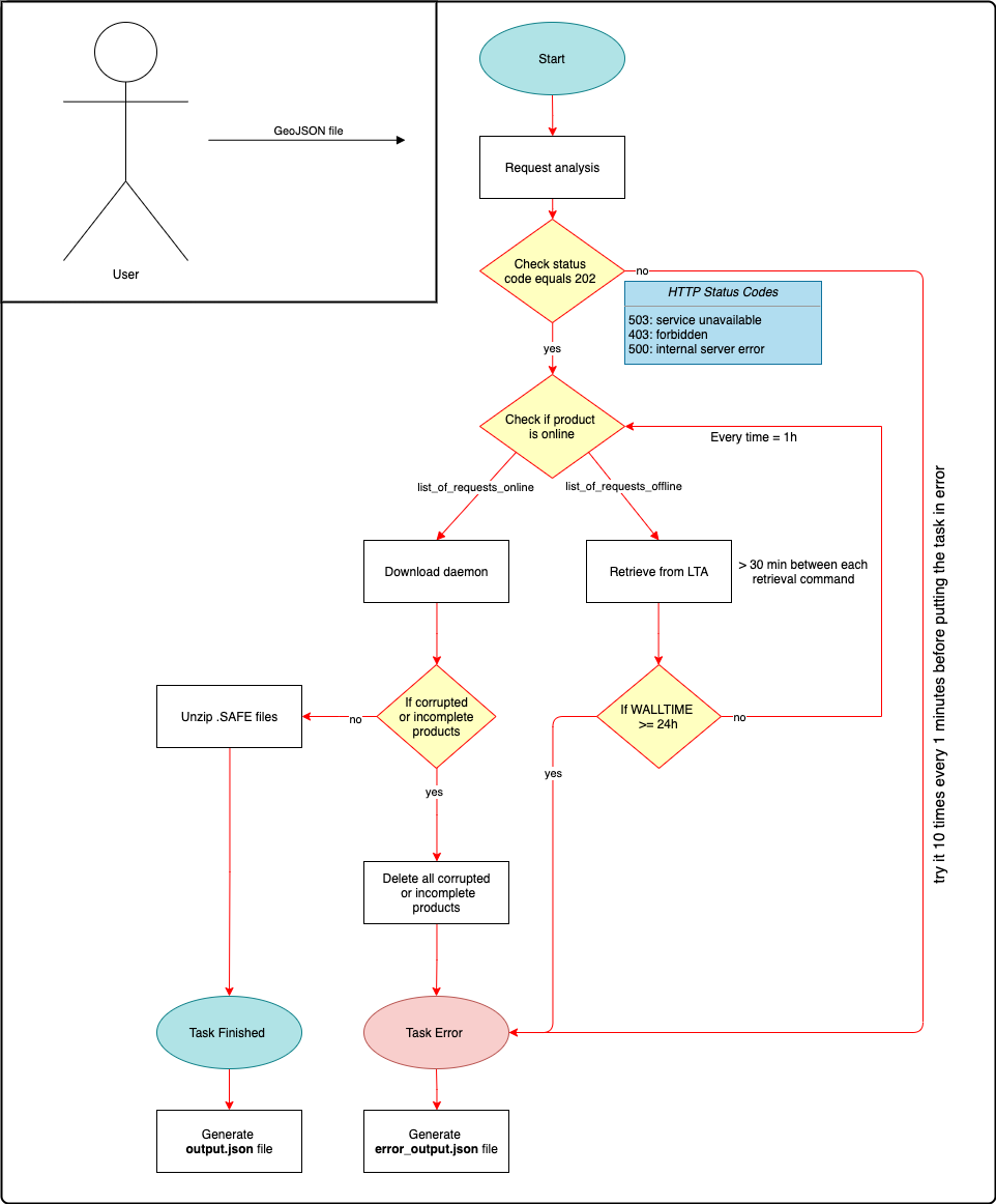
Task Variables:
Variable name |
Description |
Type |
|
Defines an engine to search and download satellite images. |
List [Copernicus, Creodias, Mundi, Onda, Peps, Sobloo and Weke, All] (default=Peps) |
|
Selects the type of data source. |
List [PA:URL,PA:URI,PA:USER_FILE,PA:GLOBAL_FILE] (default=PA:GLOBAL_FILE) |
|
Inserts a file path/name. = |
String |
|
Defines time in seconds to request an offline product from the Long Term Archive (LTA) in the Copernicus Open Access Hub’s. |
Int (default=900 seconds) |
|
Defines time in seconds to check if a product is online. |
Int (default=1800 seconds) |
|
Defines the maximum execution time of a task. |
Time (default=24:00:00) |
|
Specifies the path where the data should be downloaded. |
String |
|
Determines the policy used by the ProActive Scheduler to determine how Jobs and Tasks are scheduled. |
String |
| Please click here to create a new user account from EODAG (Earth Observation Data Access Gateway) website. |
| Please click here to create a new user account from Copernicus website. |
Note that the variables TIME_TO_RETRIEVE_IN_SECONDS, TIME_TO_CHECK_ONLINE_IN_SECONDS and WALLTIME are only valid for the Copernicus platform. In addition, it is necessary to define a policy used by the ProActive Scheduler. In this case, only two tasks must be executed simultaneously.
|
13.5.2. Fetch_Satellite_Images_From_PEPS
Task Overview: Load and return a PEPS dataset including a metadata folder with metadata files and images folder containing satellite images.
Task Variables:
Variable name |
Description |
Type |
|
Defines a town name. |
String (default=Indonesia) |
|
Specifies an instrument on a Sentinel satellite. |
List [S1, S2, S2ST, S3] (default=S2) |
|
Limits the search to a Sentinel product type. |
List [GRD, SLC, OCN (for S1) or S2MSI1C S2MSI2A S2MSI2Ap (for S2)] (default=S2MSI1C) |
|
Specifies the search to a Sentinel sensor mode. |
List [EW, IW , SM, WV (for S1) or INS-NOBS, INS-RAW (for S3)] (default=INS-NOBS) |
|
Determines a start date of the query in the format YYYYMMDD. |
String |
|
Define an end date of the query in the format YYYYMMDD. |
String |
|
Limits the search to a tile number. |
String |
|
Determines the search to a latitude in decimal degrees. |
Float |
|
Limits the search to a longitude in decimal degrees. |
Float |
|
Specifies the path where the data should be downloaded. |
String |
Please add third party credentials (USER_NAME_PEPS and USER_PASS_PEPS) in the Scheduling & Orchestration interface or Workflow Execution → Manage Third-Party Credentials to connect to PEPS.
|
| More information about the source of this task can be found here. |
13.5.3. Fetch_Satellite_Images_From_Copernicus
Task Overview: Load and return a Copernicus dataset including a metadata folder with metadata files and images folder containing satellite images according to the resolution & image band selected by user.
Task Variables:
Variable name |
Description |
Type |
|
Specifies an instrument on a Sentinel satellite. |
String [Sentinel-1, Sentinel-2, Sentinel-3, Sentinel-4, Sentinel-5, Sentinel-5, Precursor, Sentinel-6](default=Sentinel-2) |
|
Defines a geojson file with footprints of the query result. |
String |
|
Limits the search to a Sentinel product type. |
List [GRD, SLC, OCN (for S1) or S2MSI1C S2MSI2A S2MSI2Ap (for S2)] (default=S2MSI1C) |
|
Determines a start date of the query in the format YYYYMMDD. |
String |
|
Defines an end date of the query in the format YYYYMMDD. |
String |
|
If True, it uses the date defined in the START_DATE and START_DATE fields, otherwise it downloads all scenes that were published in the last 24 hours. |
Boolean (default=True) |
|
Defines granule dimensions for each resolution band. |
List [10m, 20m, 60m] (default=10m) |
|
Determines from 13 spectral bands spanning from the Visible and Near Infra-Red (VNIR) to the Short Wave Infra-Red (SWIR). |
List [All, B01, B02, B03, B04, B05, B06, B07, B08, B8A, B09, B10, B11, B12, TCI] (default=All) |
|
Specifies the path where the data should be downloaded. |
String |
Please add third party credentials (USER_NAME_COP and USER_PASS_COP) in the Scheduling & Orchestration interface or Workflow Execution → Manage Third-Party Credentials to connect to Copernicus.
|
| More information about the source of this task can be found here. |
Legal notice
Activeeon SAS, © 2007-2019. All Rights Reserved.
For more information, please contact contact@activeeon.com.